This is the multi-page printable view of this section. Click here to print.
Deep Learning
1 - Introduction
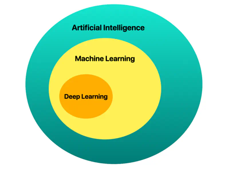
📘 Deep learning is a subset of AI and machine learning that uses multi-layered artificial neural networks to simulate human-like learning, analyzing vast data to identify complex patterns, such as recognizing objects in photos, detecting medical anomalies, or processing natural language, like LLMs.
💡 The ‘deep’ in ‘deep learning’ stands for the idea of successive layers of representations.
🐋 It is “deep” because it uses many layers (often hundreds) to automatically extract, transform, and map data features into predictions, surpassing traditional machine learning in handling unstructured data.
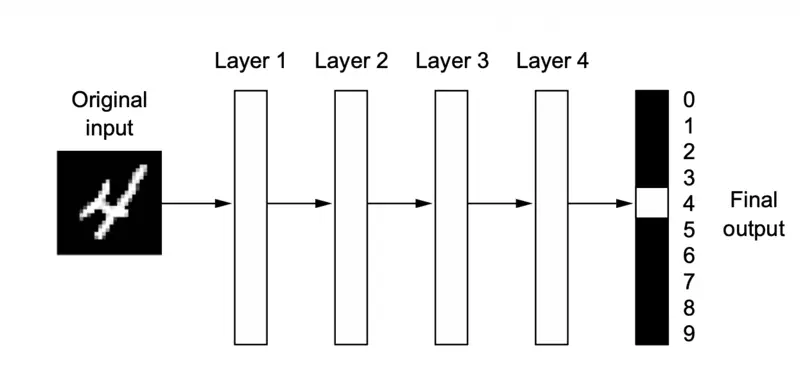
A deep neural network for digit classification
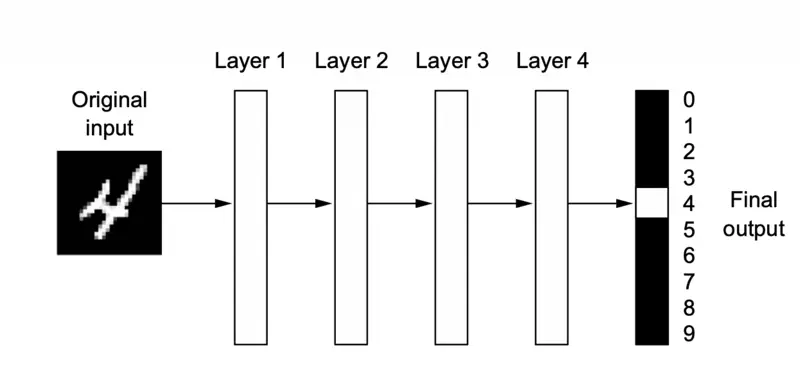
📘 Deep learning is a multistage way to learn data representations.
💡 It’s a simple idea - but, as it turns out, very simple mechanisms, sufficiently scaled, can end up looking like magic.
A fully connected neural network
Feature Engineering: Deep learning completely automates what used to be the most crucial step in a machine learning workflow, making problem-solving much easier.
Read more about Feature Engineering
Performance: Better performance for solving many kinds of problems, especially with unstructured data.
Although deep learning is a fairly old subfield of machine learning, it only rose to prominence in the early 2010s.
- Perceptron (1957), Frank Rosenblatt
- Back Propagation (1986), Geoffrey Hinton
- LSTM (1997), Sepp Hochreiter and Jürgen Schmidhuber
Some of the important algorithms such as back propagation, long short term memory (time series) of deep learning were well understood before 2000s and have barely changed since then.
Break Through Moment
It began with a win in academic image-classification competitions with GPU-trained deep neural networks.
🚀 But the watershed moment came in 2012, with the entry of Geoffrey Hinton’s group in the yearly large-scale image-classification challenge ImageNet (ImageNet Large Scale Visual Recognition Challenge, or ILSVRC for short).
ImageNet
The ImageNet challenge was very difficult at the time, consisting of classifying high-resolution color images into 1,000 different categories after training on 1.4 million
images.
- In 2011, the top-five accuracy of the winning model, based on classical approaches to computer vision, was only 74.3%.
- Then, in 2012, a team led by Alex Krizhevsky and advised by Geoffrey Hinton was able to achieve a top-five accuracy of 83.6% — a significant breakthrough.
- Since then, the competition has been dominated by deep convolutional neural networks.
Note: By 2015, the winner reached an accuracy of 96.4%, and the classification task on ImageNet was considered to be a completely solved problem.
Driving Forces
- Hardware
- Datasets and Benchmarks
- Algorithmic Advances
Note: The real bottlenecks throughout the 1990s and 2000s were data and hardware.
Experiments and Engineering
Because the deep learning field is guided by experimental findings rather than by theory, algorithmic advances only become possible when appropriate data and hardware are available to try new ideas
(or to scale up old ideas, as is often the case).
Machine learning isn’t mathematics or physics, where major advances can be done with a pen and a piece of paper.
🚀 It’s an engineering science.
Graphical Processing Unit (GPU)
Throughout the 2000s, companies like NVIDIA and AMD invested billions of dollars in developing fast, massively parallel chips (GPUs) for video games to render complex 3D scenes in real time on the computer screen.
This investment came to benefit the scientific community when, in 2007, NVIDIA launched CUDA, a programming interface for its line of GPUs.
Deep neural networks, consisting mostly of many small matrix multiplications, are also highly parallelizable using GPUs.
💡 AI is sometimes heralded as the new industrial revolution.
If deep learning is the steam engine of this revolution, then data is its coal: the raw material that powers
our intelligent machines, without which nothing would be possible.
🌐 When it comes to data, in addition to the exponential progress in storage hardware over the past 20 years (following Moore’s law), the game changer has been the rise of the internet, making it feasible to collect and distribute very large datasets for machine learning.
Today, large companies work with image datasets, video datasets, and natural language datasets that could not have been collected without the internet.
In addition to hardware and data, until the late 2000s, we were missing a reliable way
to train very deep neural networks.
As a result, neural networks were still fairly shallow, using only one or two layers
of representations; thus, they weren’t able to shine against more-refined shallow methods such as SVMs and Random Forests.
- The key issue was that of gradient propagation through deep stacks of layers.
- The feedback signal used to train neural networks would fade away as the number of layers increased.
🎯 This changed around 2009–2010 with the advent of several simple but important algorithmic improvements that allowed for better gradient propagation:
- Better activation functions for neural layers, such as ReLU.
- Better weight-initialization schemes, such as, He (2015) and Xavier initialization (2010).
- Better optimization schemes, such as RMSProp (2012) and Adam (2014).
- Advanced ways to improve gradient propagation were discovered, such as batch normalization (2015), residual connections (2015).
2 - XOR Problem
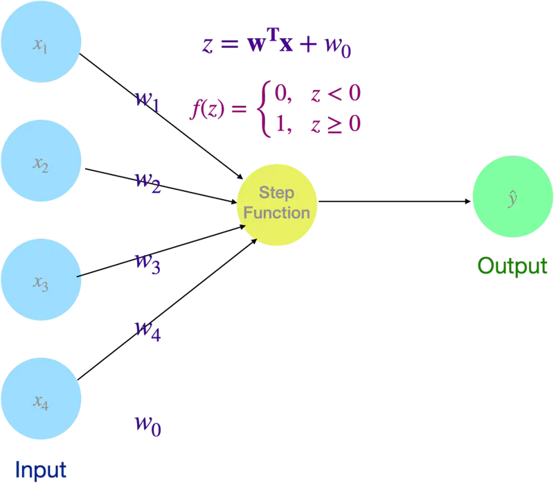
Simplest form of an artificial neural network, acting as a single-layer binary classifier that categorizes input data into one of two groups.
It serves as a mathematical model of a biological neuron, receiving multiple signals (inputs), weighting their importance, and deciding whether to ‘fire’ (output 1) or stay ‘inactive’ (output 0).
Perceptron
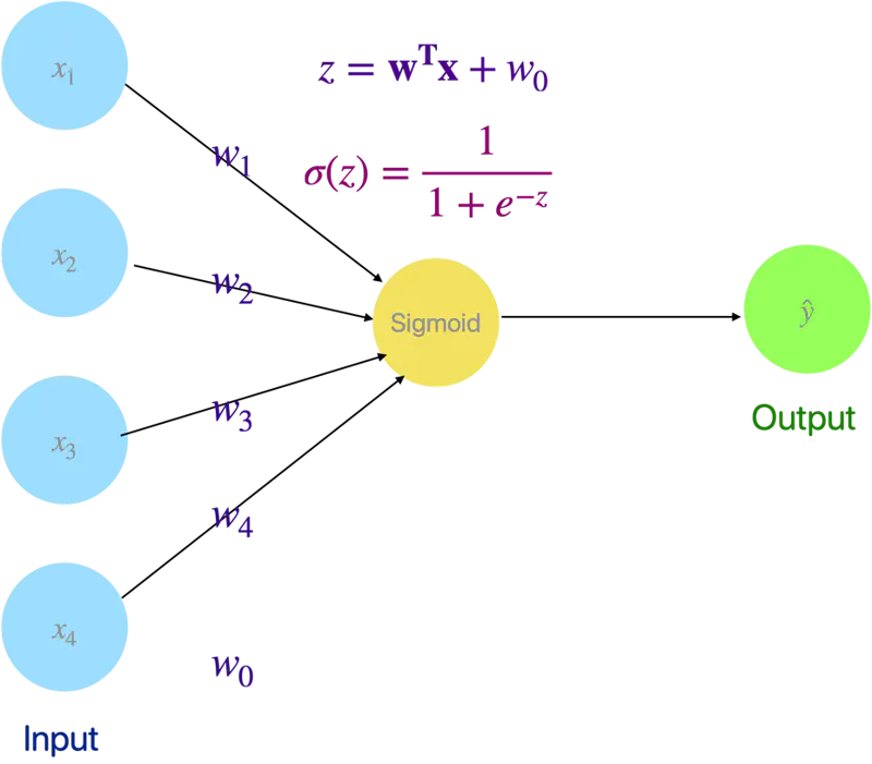
💡 Even Logistic Regression is a simple neural network with a sigmoid activation (instead of step function as in Perceptron).
Read more about Logistic Regression
Logistic Regression as a Neural Network
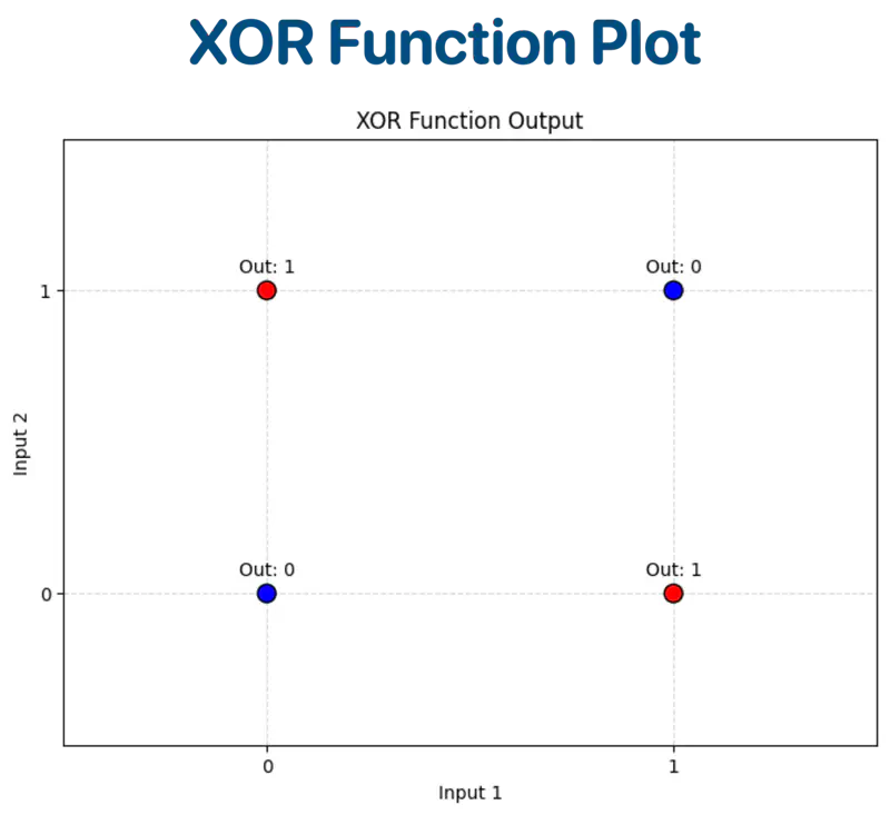
XOR Function:
| Input A | Input B | Output (A ⊕ B) |
|---|---|---|
| 0 | 0 | 0 |
| 0 | 1 | 1 |
| 1 | 0 | 1 |
| 1 | 1 | 0 |
Let’s plot the input and output on a graph for visualization.
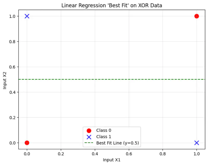
Linear Regression
The cost function:
where, \(\hat{y_i} = \mathbf{w^Tx} + w_0\)
Solving the normal equations, we get:
\(\mathbf{w = 0} , w_0 = 0.5\)
Read more about Linear Regression
This implies, whatever is the input, we always get 0.5 as output,
because linear regression is trying to fit the best line to the data, which in this case will be mid-way between the points.
And, that definitely is not the correct solution.
Logistic Regression
Similarly logistic regression can not find a single linear decision boundary to separate the 4 XOR outputs.
❌ No straight line can separate the XOR points.
Read more about Logistic Regression
Therefore, a linear model is not sufficient to represent the XOR function.
So, we need more than 1 neuron to solve the XOR problem (because logistic regression is a neural network with a single neuron).
Let’s solve the XOR problem with a simple neural network with 2 neurons (1 hidden layer) and ReLU activation function.
1 Hidden layer and 2 Neurons
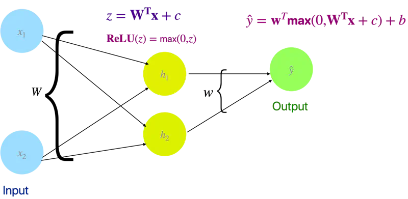
We will use linear algebra to demonstrate one of solutions to the problem.
Let input = X and output = Y.
Out of many possible solutions, let’s look at the below solution:
Weight and bias of hidden layer:
Output of hidden layer:
\[z = XW + c\]\[ XW = \begin{bmatrix} 0 & 0 \\ 0 & 1 \\ 1 & 0 \\ 1 & 1 \end{bmatrix} \begin{bmatrix} 1 & 1 \\ 1 & 1 \end{bmatrix} = \begin{bmatrix} 0 & 0 \\ 1 & 1 \\ 1 & 1 \\ 2 & 2 \end{bmatrix} \]\[ z = \begin{bmatrix} 0 & 0 \\ 1 & 1 \\ 1 & 1 \\ 2 & 2 \end{bmatrix} + \begin{bmatrix} 0 & -1 \\ 0 & -1 \\ 0 & -1 \\ 0 & -1 \end{bmatrix} = \begin{bmatrix} 0 & -1 \\ 1 & 0 \\ 1 & 0 \\ 2 & 1 \end{bmatrix} \]Now, lets apply ReLU activation function to the output ‘z’ of the hidden layer:
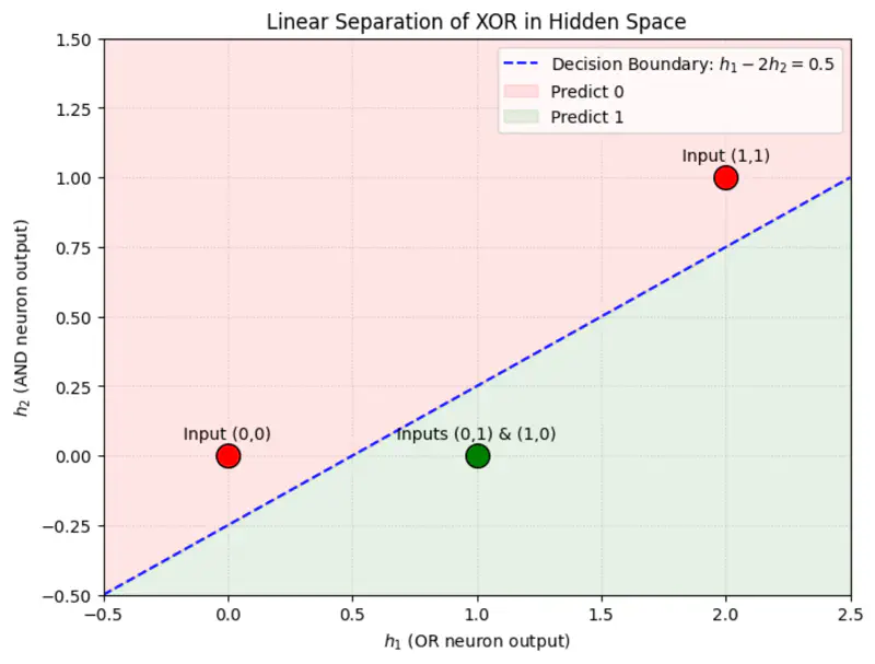
\[ReLU(z) = \begin{bmatrix} 0 & 0 \\ 1 & 0 \\ 1 & 0 \\ 2 & 1 \end{bmatrix}\]Applying ReLU non-linearity, changes the position of the points in the hidden space and now the points can be separated by a line.
Weight and bias of output layer:
\[\mathbf{w} = \begin{bmatrix} 1 \\ -2 \end{bmatrix}, \quad b = 0\]Output:
\[\hat{y} = \mathbf{w} ~ \text{max}(0, ~ XW + c) + b\]\[\hat{y} = \begin{bmatrix} 0 & 0 \\ 1 & 0 \\ 1 & 0 \\ 2 & 1 \end{bmatrix} \begin{bmatrix} 1 \\ -2 \end{bmatrix} = \begin{bmatrix} 0 \\ 1 \\ 1 \\ 0 \end{bmatrix}\]Therefore, we can see that we have got the expected output for XOR function.
import tensorflow as tf
import numpy as np

# 1. XOR Data
X = np.array([[0, 0], [0, 1], [1, 0], [1, 1]], dtype=np.float32)
y = np.array([[0], [1], [1], [0]], dtype=np.float32)

# 2. Build the Model (2 Hidden Neurons)
model = tf.keras.Sequential([
    tf.keras.layers.Dense(2, activation='leaky_relu',
                         kernel_initializer='he_normal',
                         input_shape=(2,), name='hidden_layer'),
    # Output layer (Linear for MSE)
    tf.keras.layers.Dense(1, name='output_layer')
])

print("--- Model Architecture ---")
model.summary()

# 3. Compile
model.compile(optimizer=tf.keras.optimizers.Adam(learning_rate=0.05), loss='mse')

# 4. Train
print("Training XOR Neural Network ...")
model.fit(X, y, epochs=100, verbose=0)

# 5. Extract and Print Final Weights
weights = model.get_weights()
W, c, w_out, b = weights

print("\n--- Final Weights (W) ---")
print(W)
print(f"\nHidden Bias (c): {c}")
print(f"\nOutput Weights (w): \n{w_out}")
print(f"Output Bias (b): {b}")

# 6. Predictions
print("\n--- Final Predictions ---")
preds = model.predict(X)
for i in range(len(X)):
    print(f"Input: {X[i]} | Raw Output: {preds[i][0]:.4f} | Rounded: {int(np.round(preds[i][0]))}")
Output:
--- Model Architecture ---
Model: "sequential_19"
┏━━━━━━━━━━━━━━━━━━━━━━━━━━━━━━━━━┳━━━━━━━━━━━━━━━━━━━━━━━━┳━━━━━━━━━━━━━━━┓
┃ Layer (type)                    ┃ Output Shape           ┃       Param # ┃
┡━━━━━━━━━━━━━━━━━━━━━━━━━━━━━━━━━╇━━━━━━━━━━━━━━━━━━━━━━━━╇━━━━━━━━━━━━━━━┩
│ hidden_layer (Dense)            │ (None, 2)              │             6 │
├─────────────────────────────────┼────────────────────────┼───────────────┤
│ output_layer (Dense)            │ (None, 1)              │             3 │
└─────────────────────────────────┴────────────────────────┴───────────────┘
 Total params: 9 (36.00 B)
 Trainable params: 9 (36.00 B)
 Non-trainable params: 0 (0.00 B)
Training XOR Neural Network ...

--- Final Weights (W) ---
[[-1.1186169  1.8888004]
 [ 1.0687382 -1.8048155]]

Hidden Bias (c): [-0.20543203 -0.18170778]

Output Weights (w):
[[1.3961141]
 [0.7466789]]
Output Bias (b): [0.0938225]

--- Final Predictions ---
1/1 ━━━━━━━━━━━━━━━━━━━━ 0s 105ms/step
Input: [0. 0.] | Raw Output: 0.0093 | Rounded: 0
Input: [0. 1.] | Raw Output: 1.0024 | Rounded: 1
Input: [1. 0.] | Raw Output: 0.9988 | Rounded: 1
Input: [1. 1.] | Raw Output: 0.0079 | Rounded: 0
3 - Activation Function
Real-world data (images, speech, text, financial trends) is rarely linear.
Non-linearity allows the network to learn and represent complex mappings between inputs and outputs.
- It enables the network to become a ‘Universal Function Approximator’.
A neural network with following properties can approximate any continuous function.
- at least one hidden layer
- nonlinear activation
🎯 This theorem is the mathematical reason - why neural networks are so powerful.
A deep neural network without any non-linear activation collapses into a single linear layer.
Say, if, f(x) = ax and g(x) = bx,
then, g(f(x)) = g(ax) = (ba)x = cx
where, c = ba (another constant)
Effectively, both the linear functions g(f(x)) can be represented by another single linear function h(x).
❌ So depth becomes useless.
- Sigmoid
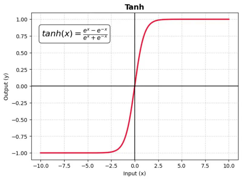
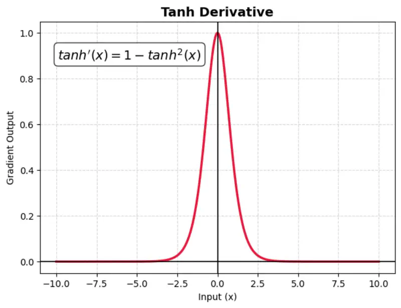
- Tanh (Hyperbolic Tangent)
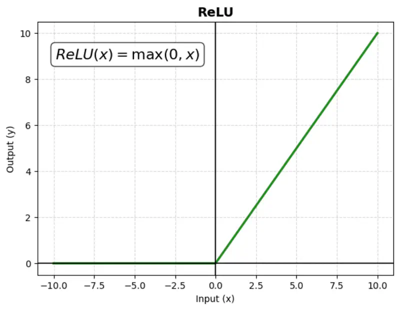
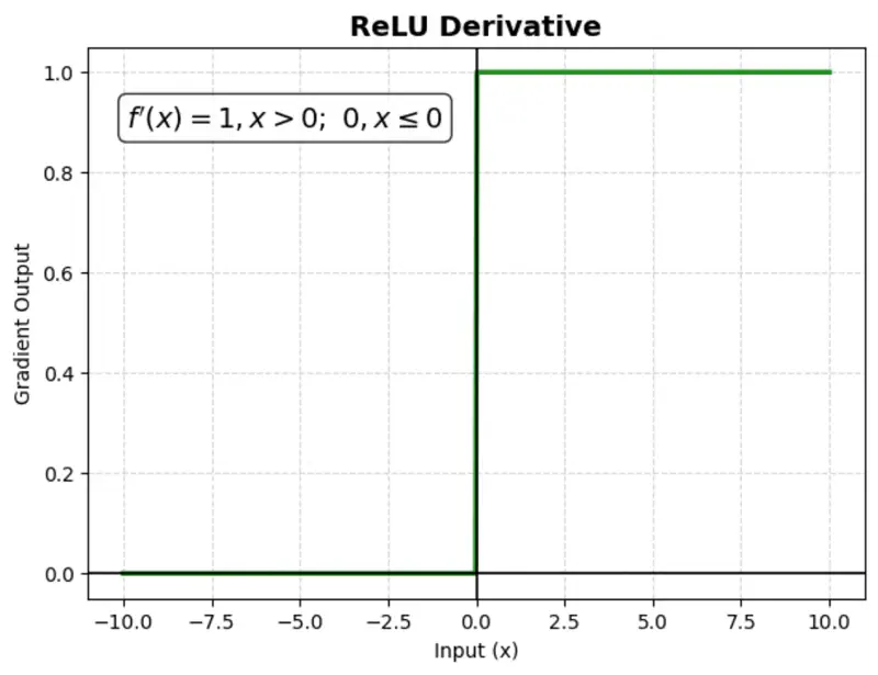
- ReLU (Rectified Linear Unit)
- Leaky ReLU
- Softmax
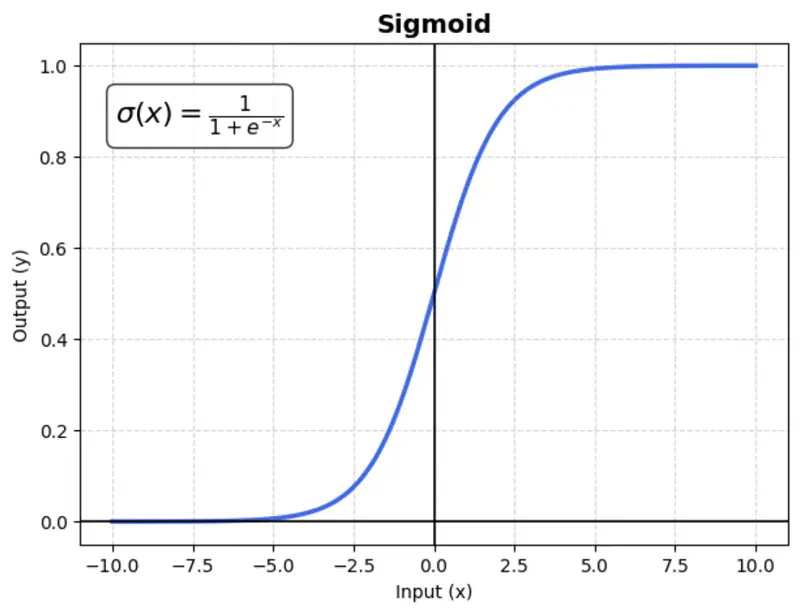
A mathematical function with a characteristic “S”-shaped curve (sigmoid curve) that maps any real-valued number into a range between 0 and 1.
\[\sigma(x) = \frac{1}{1 + e^{-x}}\]Usage:
Mostly used in binary classification output layers.
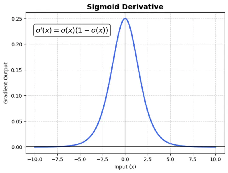
Issue:
Suffers from vanishing gradient (gradients become near-zero for high or low input values), which slows down training.
A mathematical function with a S-shaped curve that maps any real-valued number into a range between -1 and 1.
It is zero-centered, making it more effective than the sigmoid function for hidden layers in neural networks.
Benefit:
Makes optimization faster as the data is zero-centered.
Issue:
TanH also suffers from vanishing gradient (gradients become near-zero for high or low input values), which slows down training.
A mathematical function that outputs the input value directly if it is positive, and zero otherwise.
Computationally simple; very fast to compute; does not saturate in the positive direction.
Benefit:
It is computationally efficient and helps mitigate the ‘vanishing gradient’ problem, making it the most popular choice for hidden layers.
Issue:
‘Dying ReLU’ problem: negative inputs result in a zero gradient, meaning the neuron stops learning (no weight updates).
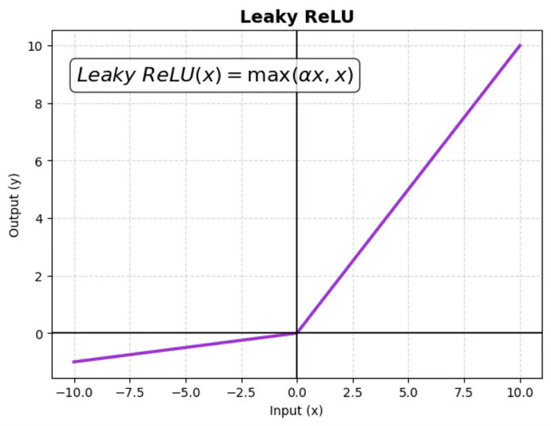
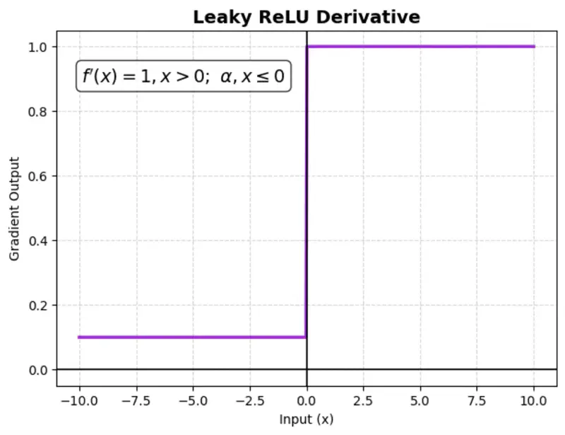
Instead of setting negative input values to zero like a standard ReLU, Leaky ReLU allows a small,
non-zero gradient (slope) for negative values.
This ensures that neurons continue learning (even for negative values).
where ‘\(\alpha\)’ is a small constant (e.g., 0.01)
Benefit:
Fixes the ‘dying ReLU’ problem.
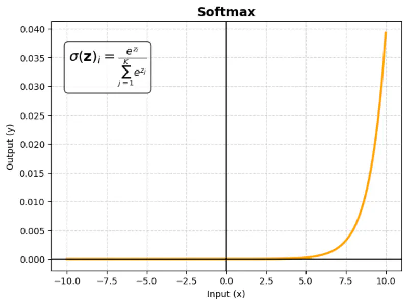
Multivariate activation function that takes a vector of raw scores (logits) and converts them into a probability distribution; sum of probabilities = 1.
\[\sigma(\mathbf{z})_i = \frac{e^{z_i}}{\sum_{j=1}^K e^{z_j}}\]where ‘K’ = number of classes
Winner Takes Most
Since, the exponential function \(e^{x}\) grows rapidly.
A small lead in raw score (logit) results in a disproportionately large share of the final probability.
So, winner takes the majority share, but non-winners still retain a small, non-zero probability.
Role of Temperature (\(T\))
The “sharpness” of the distribution is controlled by a temperature parameter \(T\):
- High Temperature (\(T \to \infty\)): The output becomes a uniform distribution, where all classes have nearly equal probability regardless of their input scores.
- Low Temperature (\(T \to 0\)): The output becomes a “hard” max (one-hot vector), where the highest score gets a probability of \(1\) and all others \(0\).
Gradient of Softmax
\[\frac{\partial \sigma_i}{\partial z_j} = \begin{cases} \sigma_i(1 - \sigma_i) & \text{if } i = j \\ -\sigma_i\sigma_j & \text{if } i \neq j \end{cases} \]Combining both cases:
\[\frac{\partial \sigma_i}{\partial z_j} = \sigma_i (\delta_{ij} - \sigma_j)\]where, \(\delta_{ij}\) is the Kronecker delta (1 if \(i=j\) (diagonal), 0 otherwise).
Usage:
- Almost exclusively used in the output layer of multi-class classification networks.
- Attention score calculation.
Softmax Graph
Example
Consider an AI model reading a product review to categorize the customer’s mood into three classes:
Positive,Neutral, or Negative.
| Class | Score (Logit) | Softmax |
|---|---|---|
| Positive | 3 | 82.1% |
| Neutral | 1 | 11.1% |
| Negative | 0.5 | 6.7% |
Similarly, you can calculate for negative and neutral sentiments.
4 - Optimization Method
The loss function surface in deep learning is non-convex, i.e, it has multiple local minima, saddle points,
and plateaus rather than a single, global minimum.
So, in the context of neural network training, we usually do not care about finding the exact (global) minimum of a function,
but seek only to reduce its value sufficiently to obtain good generalization error.
Non-Convex Loss Surface Examples
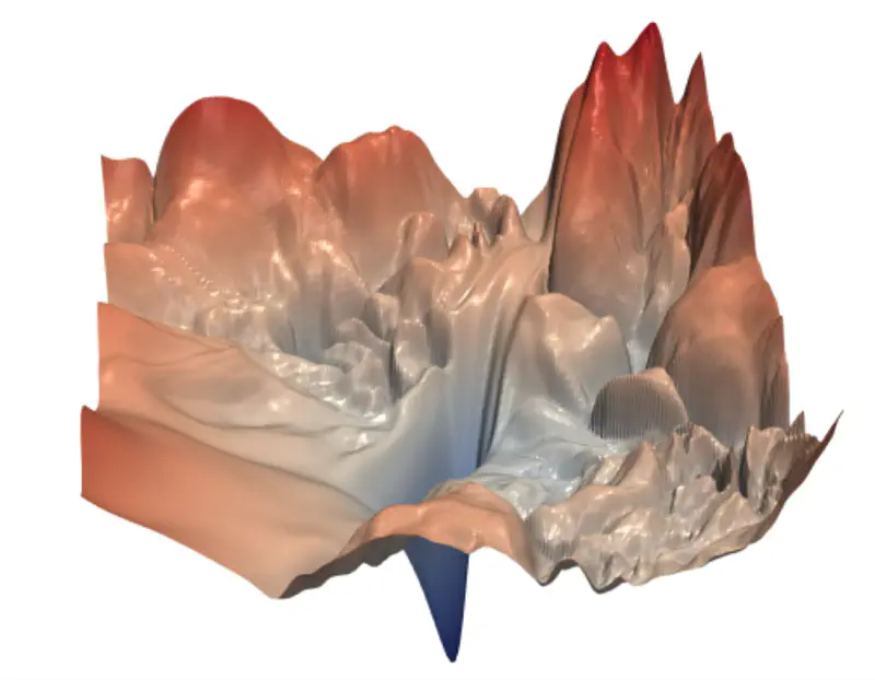
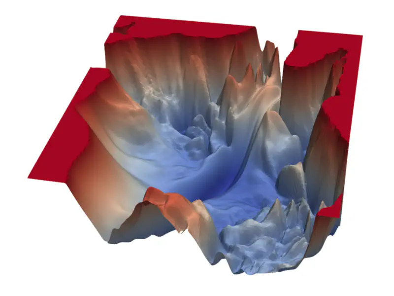
Because of the non-convex loss surface, convergence to a good minimum is often slow, because of multiple reasons:
- Multiple local minima; may not land in a good enough local minima.
- Saddle points; near a saddle point, optimizer barely moves.
- Presence of flat regions (plateaus), where the gradient is near zero, offering minimal guidance for the optimizer.
- “Ravine-like” structure (steep on one side, flat on the other), stochastic gradient descent oscillates uncontrollably.
- Different parameters require different learning rates; e.g, sparse parameters will get very few updates.
Training deep neural networks is inherently complex because of the multiple layers and the vast number of parameters to be updated during training.
Therefore, we need to find ways to accelerate the optimization process.
The optimization process can be accelerated considerably by using stochastic gradient descent (instead of simple gradient descent), i.e, follow the gradient of randomly selected mini-batches downhill.
\[w_{new} = w_{old} - \eta.\text{(average gradient of randomly chosen ‘m' data points)}\]where, \(\eta\) = learning rate
In practice, it is common to decay the learning rate linearly until some pre-defined fixed number of iterations ‘\(\tau\)’.
The primary reason for this approach is to start with a high learning rate to rapidly traverse the loss landscape and escape poor local minima, while later using a small learning rate to fine-tune the parameters and settle into a deeper, more stable minimum without oscillating around it.
\[\eta_k = (1-\alpha)\eta_0 + \alpha\eta_{\tau}\]where, \(\alpha = \frac{k}{\tau}\)
After,’\(\tau\)’ iterations, leave the learning rate \(\eta\) constant.
e.g., \(\eta_0 = 0.1,~ \eta_{\tau}=0.01, \text{ and } \tau=100\)
Say, we have ’n’ samples, and we divide them into mini-batches, such that, each mini-batch has ‘m’<’n’ samples.
- 1 iteration = weight update after computing the gradient of 1 mini-batch
- 1 epoch = one complete pass through the entire training dataset = n/m iterations
- L epochs = L x (n/m) iterations
Note:
- Size ‘m’ of a mini-batch is decided based on the computing resources, such as RAM, GPU, TPU etc., e.g, Nvidia H100 GPU has 80GB RAM.
- In practice, the mini-batch size is chosen to be the largest possible power of 2 that fits within the available GPU memory while still allowing for good model performance.
- Samples in the mini-batches are randomized in every epoch.
Methods to accelerate the optimization process in deep learning:
- Momentum Based; Polyak (1964) | Refined for Deep Learning: Sutskever et al. (2013)
- AdaGrad (Adaptive Gradient); Duchi, Hazan, and Singer (2011)
- RMSProp (Root Mean Square Propagation); Geoffrey Hinton (2012)
- Adam (Adaptive Moment Estimation); Kingma and Ba (2014)
💡 Momentum introduces velocity.
(term borrowed from Physics, where momentum = mass x velocity)
‘Accumulates’ velocity in directions of consistent gradients and cancels out directions that fluctuate.
Algorithm
- For each iteration (t):
- Instead of moving purely by gradient: \[w_{t+1} = w_{t} - \eta . g_t\]
- Accumulate previous gradients, i.e, the velocity (speed + direction): \[ v_{t} = \gamma . v_{t-1} + \eta. g_t\]
- where, \( \gamma \) = momentum coefficient (typically 0.9)
- Update parameter: \[ w_{t+1} = w_{t} - v_{t} \]
Size of the step depends on how large and how aligned are a sequence of gradients.
\[ \begin{aligned} \text{Let, } v_0 &= 0 \\ v_1 &= \gamma. v_0 + \eta.g_0 = \eta.g_0\\ v_2 &= \gamma. v_1 + \eta.g_1 = \gamma (\eta.g_0) + \eta.g_1 \\ v_3 &= \gamma. v_2 + \eta.g_2 = \gamma (\gamma (\eta.g_0) + \eta.g_1 ) + \eta.g_2 = \eta(\gamma^2 g_0 + \gamma g_1 + g_2)\\ v_{k} &= \eta(\gamma^{k-1} g_0 + \gamma^{k-2} g_1 + \dots g_{k-1})\\ \end{aligned} \]If many successive gradients point in exactly the same direction, then we want to take larger steps.
\[ \lim_{k\rightarrow \infty} v_k = \eta.g(1+\gamma+ \gamma^2 + \dots \infty) \]The term inside the bracket, is a geometric progression with the common ratio \(\gamma < 1\).
So, if the momentum algorithm always observes gradient ‘g’, then it will accelerate in the direction of ‘g’, until reaching a terminal velocity where the size of each step is:
\[ \frac{\eta. \lVert g \rVert}{1-\gamma} \]where, \(0 < \gamma < 1\)
Say, if \(\gamma\)= 0.9, then it means to multiply the maximum velocity by 10 relative to a gradient descent algorithm.
Momentum Based Optimizer Vs SGD
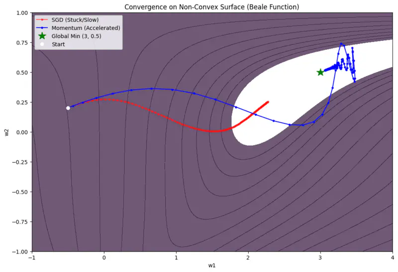
Limitations
- Momentum can be like a heavy ball rolling down a hill; it gathers so much speed that it may overshoot the minima.
- It does not adjust the learning rate based on the importance of specific features.
💡 Scales the learning rate for each parameter based on the historical sum of squares of its gradients.
Problem
In many datasets, some features are frequent while others are sparse.
e.g., Predicting house prices based on certain rare feature, such as, presence of shopping mall.
For most of the houses the value of that feature is 0.
A single learning rate ‘\(\eta\)’ for all parameters is inefficient.
We want larger updates for sparse features and smaller updates for frequent ones.
Algorithm
- For each iteration (t):
- Calculate gradient \(g_t\).
- Accumulate gradients: \[ r_{t} = r_{t-1} + g_t \odot g_t\]
- Update parameter: \[ w_{t+1} = w_{t} - \frac{\eta}{\sqrt{r_t} + \delta} \odot g_t \]
- where, \(\delta\) is small smoothing term (e.g. \(10^{-8}\)) to avoid division by 0.
- if, \(g = \begin{bmatrix} g_1 \\ g_2 \\ \vdots \\ g_d \end{bmatrix} \), then \( g \odot g = \begin{bmatrix} g_1^2 \\ g_2^2 \\ \vdots \\ g_d^2 \end{bmatrix} \) (element wise dot product)
Since, \(r_{t+1} = r_{t} + g_t \odot g_t\), so, for sparse features, we hardly get any gradient updates, so ‘g’ is mostly 0.
Therefore, accumulations ‘r’ is very small.
Since, \(w_{t+1} = w_{t} - \frac{\eta}{\sqrt{r_t} + \delta} \odot g_t\), this implies that, the learning rate is inversely proportional to accumulations ‘r’.
Therefore, sparse features get larger updates, whereas, for weights that are frequent will have very large accumulations,
as a result, the learning rate will start decaying.
Limitation
Vanishing Learning Rate Problem:
Since accumulation of gradients increases monotonically.
This causes the effective learning rate to shrink until it becomes infinitesimally small, effectively ‘killing’
the learning process before the model converges.
💡 Instead of summing all past squared gradients, as in AdaGrad, RMSProp uses an exponentially decaying average to discard history from the extreme past so that it can converge rapidly.
Algorithm
- For each iteration (t):
- Calculate gradient \(g_t\).
- Accumulate gradients: \[ r_{t} = \rho r_{t-1} + (1 - \rho)g_t \odot g_t \]
- Update parameter: \[ w_{t+1} = w_{t} - \frac{\eta}{\sqrt{r_t} + \delta} \odot g_t \]
- where, \(\delta\) is small smoothing term (e.g. \(10^{-8}\)) to avoid division by 0.
- if, \(g = \begin{bmatrix} g_1 \\ g_2 \\ \vdots \\ g_d \end{bmatrix} \), then \( g \odot g = \begin{bmatrix} g_1^2 \\ g_2^2 \\ \vdots \\ g_d^2 \end{bmatrix} \) (element wise dot product)
Since, \(r_{t} = \rho r_{t-1} + (1 - \rho)g_t \odot g_t\), say, if \(\rho = 0.9\), then we trust the historical average 90% and the new gradient only 10%, i.e, \(r_t = 0.9r_{t-1} + 0.1g_t \odot g_t\). \[ r_t = (1-\rho)g_t^2 + \rho(1-\rho)g_{t-1}^2 + \rho^2(1-\rho)g_{t-2}^2 + \dots\]
So, if the algorithm always observes gradient ‘g’, then \(r_t\) becomes:
\[ r_t = (1-\rho)g^2 (1 + \rho + \rho^2 + \dots)\]The term inside the second bracket, is a geometric progression with the common ratio \(\rho < 1\).
Note: \(\rho \) is the decay rate (commonly 0.9 or 0.99).
So, the accumulation of gradient does not grow uncontrollably, as in AdaGrad.
Therefore, the “Vanishing Learning Rate” problem is solved.
Limitation
Lacks the ‘momentum’ component to accelerate through flat regions or dampen oscillations.
💡Adam optimizer combines:
- Adaptive learning rates of RMSProp
- Accelerated convergence of Momentum
Adam calculates an exponential moving average of the gradient (first moment) and the squared gradient (second moment).
It also includes a bias-correction term to account for the fact that these averages are initialized at zero.
Algorithm
- For each iteration (t):
- Calculate gradient \(g_t\).
- Update biased first moment estimate: \[ m_t = \beta_1 m_{t-1} + (1 - \beta_1)g_t \]
- Update biased second raw moment estimate: \[ v_t = \beta_2 v_{t-1} + (1 - \beta_2)g_t^2 \]
- Compute bias-corrected first moment estimate: \[ \hat{m}_t = \frac{m_t}{1 - \beta_1^t} \]
- Compute bias-corrected second raw moment estimate: \[ \hat{v}_t = \frac{v_t}{1 - \beta_2^t} \]
- Update parameter: \[w_{t+1} = w_t - \frac{\eta}{\sqrt{\hat{v}_t} + \epsilon} \hat{m}_t\]
Since, \(m_t = \beta_1 m_{t-1} + (1 - \beta_1)g_t\), say if, \(\beta_1 = 0.9\), then we trust the historical average 90% and the new gradient only 10%, i.e, \(m_t = 0.9m_{t-1} + 0.1g_t\)
Expanding the equation:
\[ m_t = 0.1g_t + 0.9(0.9 m_{t-2} + 0.1 g_{t-1}) = 0.1g_t + 0.09 g_{t-1} + 0.081 g_{t-2} + \dots \]Because the weight drops by a factor of \(\beta_1\) for every step back, the influence of older gradients decays exponentially.
Bias Correction
Bias correction compensates for the fact that the initial estimates of the first and second moments are biased towards zero.
Since \(m_0\) is initialized to zero, \(m_t\) will be close to zero during the initial time steps, especially when \(\beta_1\) is close to 1.
Common defaults: \(\beta_1 = 0.9 ,~ \beta_2 = 0.999,~ \eta = 0.001\)
Advantages
✅ Faster convergence.
✅ Require little to no adjustment of its default hyper-parameter values.
✅ It is computationally efficient, requires little memory to store moving averages.
✅ Adam is currently the ‘default’ optimizer for most deep learning tasks.
5 - Regularization
In ‘Deep Learning’ before thinking of regularization we make sure that the model is able to overfit on the training data
and then later take steps to prevent overfitting.
Overfitting on training data ensures that the model training is successful and is not under-fit, i.e:
- No coding error.
- Layers are all connected and have sufficient capacity to learn the complexity in data.
- Initialization parameters of gradient descent are fine, so that convergence to a local minima occurs.
- Model is trained for enough iterations/epochs.
Note: Overfitting on training data => very low training loss.
Once, we have made sure that the deep learning model is overfitting, now we test the model performance against a separate validation dataset, and if the performance on validation set is poor, this implies that:
- Training and Validation data distributions are different, or
- Overfitting on training data.
Data Augmentation
The best way to make a machine learning model generalize better is to train it on more data.
Of course, in practice, the amount of data we have is limited.
One way to get around this problem is to create fake data from the existing data and add it to the training set.Regularization
- L2 Regularization (Weight Decay)
- Early Stopping
- Dropout
Adds a penalty term proportional to the square of the magnitude of weights to the loss function.
- It prevents overfitting by forcing weight values to be small, encouraging a smoother, simpler model that generalizes better to new data.
- Weights ‘decay’ toward zero at every step, which is why it’s often called ‘Weight Decay’. \[ \underset{w}{\mathrm{min}}\ J_{reg}(w) = \underset{w}{\mathrm{min}}\ J(w) + \lambda.\sum_{j=1}^n \Vert w_j \Vert_2^2 \]
Note: Most modern optimizers (like AdamW) implement this by default to keep weights small and prevent overfitting.
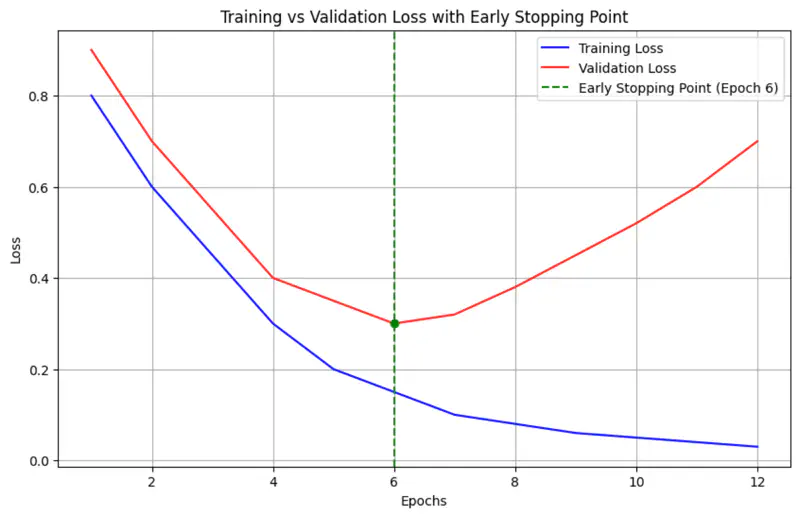
Early stopping is a ‘free’ regularization technique that relies on monitoring the model’s performance on a separate validation set during training.
As training progresses, the error on both training and validation sets usually decreases.
However, at some point, the model begins to ‘memorize’ the training data.
While the training error continues to drop, the validation error starts to rise.
Early stopping halts the training at the precise moment the validation error is at its minimum.
- e.g. if validation loss does not improve for 5 epochs, stop training.
Code
# 1. Define the EarlyStopping callback
# Monitors 'val_loss' and stops if no improvement for 3 epochs.
# restore_best_weights=True ensures you get the model from the best epoch.
early_stop_callback = EarlyStopping(
    monitor='val_loss',
 patience=3,
    restore_best_weights=True
)

# 2. Create a simple model
model = Sequential([
    Dense(10, activation='relu', input_shape=(5,), name="hidden_1", kernel_initializer="he_normal"),
    Dense(1, activation='sigmoid', name="output")
])
model.compile(optimizer='adam', loss='binary_crossentropy', metrics=['accuracy'])


# 3. Train the model with the EarlyStopping callback
# The 'callbacks' argument accepts a list of callbacks.
history = model.fit(
    X_train, y_train,
    epochs=100, # Set a large number of epochs
    validation_data=(X_val, y_val),
 callbacks=[early_stop_callback], # Pass the callback here
    verbose=1
)
Output
Epoch 22/100
4/4 ━━━━━━━━━━━━━━━━━━━━ 0s 23ms/step - accuracy: 0.6100 - loss: 0.6458 - val_accuracy: 0.6000 - val_loss: 0.7082
Epoch 23/100
4/4 ━━━━━━━━━━━━━━━━━━━━ 0s 23ms/step - accuracy: 0.6200 - loss: 0.6450 - val_accuracy: 0.6000 - val_loss: 0.7076
Epoch 24/100
4/4 ━━━━━━━━━━━━━━━━━━━━ 0s 23ms/step - accuracy: 0.6200 - loss: 0.6450 - val_accuracy: 0.6000 - val_loss: 0.7070
Epoch 25/100
4/4 ━━━━━━━━━━━━━━━━━━━━ 0s 23ms/step - accuracy: 0.6200 - loss: 0.6449 - val_accuracy: 0.6000 - val_loss: 0.7079
Epoch 26/100
4/4 ━━━━━━━━━━━━━━━━━━━━ 0s 23ms/step - accuracy: 0.6200 - loss: 0.6446 - val_accuracy: 0.6000 - val_loss: 0.7089
Epoch 27/100
4/4 ━━━━━━━━━━━━━━━━━━━━ 0s 24ms/step - accuracy: 0.6200 - loss: 0.6447 - val_accuracy: 0.6000 - val_loss: 0.7094
Training stopped early after 27 epochs.
Ensemble
Ensemble models reduce overfitting by combining the predictions of multiple diverse models, which reduces the overall
variance of the final model.
Note: If variance of each model is \(\sigma^2 \) then the combined variance of ensemble will be \(\frac{\sigma^2}{k}\).
Read more about Average Variance of Ensemble
Problem
But training multiple different ‘deep learning’ models is costly, also at runtime we need to get the predictions from
all ‘k’ models and take the average of them, which may be time-consuming.
💡 Dropout provides an inexpensive approximation to training and running an ensemble of models.
Randomly remove non-output neurons, i.e, input or hidden layer neurons from the network during every mini-batch (only for that mini-batch) training.
Note: Possible subnetworks = \(2^{n}\), where ’n’ is number of neurons in the input and hidden layers.
Research Paper: Improving neural networks by preventing co-adaptation of feature detectors, Hinton et al., 2012, https://arxiv.org/pdf/1207.0580
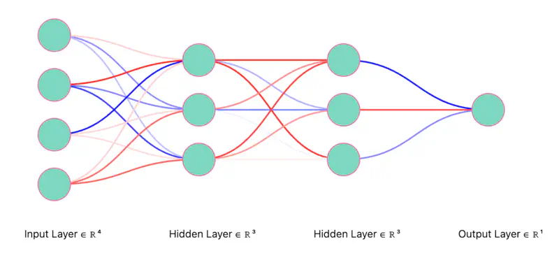
Let’s understand Dropout using the example below.
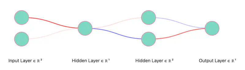
We will start with a fully connected neural network and randomly dropout(turn-off) neurons.
Fully Connected Neural Network
Dropout Neurons Randomly (iteration 1)
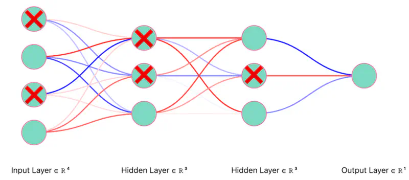
Thinned Network (iteration 1)
Note: Only the “weights” corresponding to retained neurons will be updated in each iteration (mini-batch).
Dropout Neurons Randomly (iteration 2)
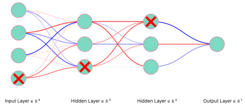
Thinned Network (iteration 2)
Note: Only the “weights” corresponding to retained neurons will be updated in each iteration (mini-batch).
Since, all neurons are not present in every iteration, so all the weights will not be updated, thus preventing over-fitting.
- We can think of removal of hidden neurons as adding some form of random noise to features.
- Removal of input neurons as input variations.
- All of the above things prevent over-fitting.
Say probability of retaining a neuron,
p(hidden neuron) = 0.6 and p(input neuron) = 0.8
Generate a random number \(r_i \in [0,1]\), if \(r_i \le 0.8\), then retain the input neuron, else drop it; this corresponds to a 80% retention probability.
Co-adaptation in deep learning occurs when neurons become overly dependent on others to correct errors, leading to fragile, overfitted models that perform poorly on new data.
💡 Dropout prevents co-adaptation.
- No single neuron can rely on the presence of another specific neuron to correct its errors.
- This forces every neuron to learn features independently.
Since, each neuron is present in the network with probability ‘p’, so the corresponding outgoing weights of the neuron are scaled by the factor ‘p’ to account for the presence of the that neuron in the network during training.
💡 At inference time we scale the weights.
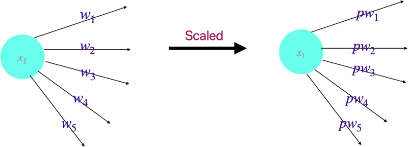
Note: No clear justification for doing this.
import tensorflow as tf
from tensorflow.keras import layers, regularizers, models
import numpy as np

# Create some dummy data for demonstration purposes
X_train = np.random.rand(1000, 32)
y_train = np.random.rand(1000, 1)
X_val = np.random.rand(200, 32)
y_val = np.random.rand(200, 1)

# Define the L2 regularization strength (e.g., 0.0001)
l2_strength = 1e-4

# Create a Sequential model with L2 regularization and Dropout layers
model = models.Sequential([
    # Add a Dense layer with L2 regularization
    layers.Dense(128, activation='relu',
              kernel_regularizer=regularizers.l2(l2_strength),
                 input_shape=(32,)),

    # Add a Dropout layer with a dropout rate of 30%
 layers.Dropout(0.3),

    # Another Dense layer with L2 regularization
    layers.Dense(64, activation='relu',
                 kernel_regularizer=regularizers.l2(l2_strength)),

    # Another Dropout layer with a dropout rate of 20%
 layers.Dropout(0.2),

    # Output layer
    layers.Dense(1, activation='linear')
])

# Compile the model
model.compile(optimizer='adam',
              loss='mse', # Using Mean Squared Error loss for a regression example
              metrics=['mae']) # Mean Absolute Error as a metric

# Display the model summary
model.summary()

# Train the model (optional, for a complete example)
# history = model.fit(X_train, y_train, epochs=10, validation_data=(X_val, y_val), verbose=1)
Output
------Model Architecture-------
Model: "sequential_21"
┏━━━━━━━━━━━━━━━━━━━━━━━━━━━━━━━━━┳━━━━━━━━━━━━━━━━━━━━━━━━┳━━━━━━━━━━━━━━━┓
┃ Layer (type)                    ┃ Output Shape           ┃       Param # ┃
┡━━━━━━━━━━━━━━━━━━━━━━━━━━━━━━━━━╇━━━━━━━━━━━━━━━━━━━━━━━━╇━━━━━━━━━━━━━━━┩
│ dense_3 (Dense)                 │ (None, 128)            │         4,224 │
├─────────────────────────────────┼────────────────────────┼───────────────┤
│ dropout_2 (Dropout)             │ (None, 128)            │             0 │
├─────────────────────────────────┼────────────────────────┼───────────────┤
│ dense_4 (Dense)                 │ (None, 64)             │         8,256 │
├─────────────────────────────────┼────────────────────────┼───────────────┤
│ dropout_3 (Dropout)             │ (None, 64)             │             0 │
├─────────────────────────────────┼────────────────────────┼───────────────┤
│ dense_5 (Dense)                 │ (None, 1)              │            65 │
└─────────────────────────────────┴────────────────────────┴───────────────┘
 Total params: 12,545 (49.00 KB)
 Trainable params: 12,545 (49.00 KB)
 Non-trainable params: 0 (0.00 B)
6 - Batch Normalization
Problem
In deep neural networks, during training, as weights update the distribution of input values to hidden layers changes
continuously, also called, ‘internal covariate shift’ (ICS).
This change forces layers to constantly adapt to new input distributions, which :
- slows down training,
- hinders convergence, and
- makes hyper-parameter tuning difficult
A deep neural network for digit classification
Batch Normalization is a technique to control the variation in the features, such that, they do not vary too much and are bounded (by normalizing the inputs to each layer).
\[ \hat{x}_i = \frac{x_i - \mu_{\mathcal{B}}}{\sqrt{\sigma_{\mathcal{B}}^2 + \epsilon}} \]where, \(\epsilon \approx 10^{-5}\) is a tiny constant to prevent division by zero.
If we always normalize to mean \(\mu\)=0 and variance \(\sigma^2\)=1, we might restrict the layer too much (e.g., forcing everything into the linear region of a Sigmoid function) and the network might lose representational power.
💡 So BatchNorm introduces learnable parameters:
\[y_i = \gamma \hat{x}_i + \beta\]- \(\gamma\) = scaling parameter
- \(\beta\)= shifting parameter
Note: The network can now decide for itself if it wants the mean(\(\mu\)) to be 0 and variance(\(\sigma^2\)) to be 1.
If the optimal state for the network is something else, it can learn the values for ‘\(\gamma\)’ and ‘\(\beta\)’ to undo the normalization.
Inference Time
- During training, mean(\(\mu\)) and variance(\(\sigma^2\)) come from current mini-batch.
- At inference (test) time, we use frozen running averages of the mean(\(\mu\)) and variance(\(\sigma^2\)) calculated during training.
Research Paper: Batch Normalization: Accelerating Deep Network Training by Reducing Internal Covariate Shift, Ioffe & Szegedy, 2015, https://arxiv.org/pdf/1502.03167
- Mitigates changing distributions (internal covariate shift).
- Prevents vanishing/exploding gradients.
- Allows for higher learning rates.
- Smoothing the optimization landscape.
- Acts as a regularizer to reduce overfitting.
- Because BN calculates the mean(\(\mu\)) and variance(\(\sigma^2\)) for each mini-batch, these statistics vary slightly across different batches. This randomness introduces a small amount of noise into the activations, which acts as a regularizer, similar to dropout.
import tensorflow as tf
from tensorflow.keras import layers, models, regularizers
import numpy as np

# 1. Setup Synthetic Data (Binary Classification)
# 1000 samples, 20 features per sample
X = np.random.rand(1000, 20).astype(np.float32)
y = np.random.randint(2, size=(1000, 1)).astype(np.float32)

# 2. Define the Sequential Model
model = models.Sequential([
    # Input Layer
    layers.Input(shape=(20,)),

    # Hidden Layer 1: Dense + L2 Regularization
    layers.Dense(64, kernel_regularizer=regularizers.l2(0.01), name="dense_1"),
    layers.BatchNormalization(name="batch_norm_1"), # Normalizes activations
    layers.Activation('relu'),
    layers.Dropout(0.3, name="dropout_1"),          # Prevents overfitting

    # Hidden Layer 2
    layers.Dense(32, kernel_regularizer=regularizers.l2(0.01), name="dense_2"),
    layers.BatchNormalization(name="batch_norm_2"),
    layers.Activation('relu'),
    layers.Dropout(0.2, name="dropout_2"),

    # Output Layer (Sigmoid for binary probability)
    layers.Dense(1, activation='sigmoid', name="output_layer")
])

# 3. Compile the Model
model.compile(
    optimizer=tf.keras.optimizers.Adam(learning_rate=0.001),
    loss='binary_crossentropy',
    metrics=['accuracy']
)

# 4. Print Architecture & Parameters
print("--- Model Architecture ---")
model.summary()
Output
--- Model Architecture ---
Model: "sequential_23"
┏━━━━━━━━━━━━━━━━━━━━━━━━━━━━━━━━━┳━━━━━━━━━━━━━━━━━━━━━━━━┳━━━━━━━━━━━━━━━┓
┃ Layer (type)                    ┃ Output Shape           ┃       Param # ┃
┡━━━━━━━━━━━━━━━━━━━━━━━━━━━━━━━━━╇━━━━━━━━━━━━━━━━━━━━━━━━╇━━━━━━━━━━━━━━━┩
│ dense_1 (Dense)                 │ (None, 64)             │         1,344 │
├─────────────────────────────────┼────────────────────────┼───────────────┤
│ batch_norm_1                    │ (None, 64)             │           256 │
│ (BatchNormalization)            │                        │               │
├─────────────────────────────────┼────────────────────────┼───────────────┤
│ activation_2 (Activation)       │ (None, 64)             │             0 │
├─────────────────────────────────┼────────────────────────┼───────────────┤
│ dropout_1 (Dropout)             │ (None, 64)             │             0 │
├─────────────────────────────────┼────────────────────────┼───────────────┤
│ dense_2 (Dense)                 │ (None, 32)             │         2,080 │
├─────────────────────────────────┼────────────────────────┼───────────────┤
│ batch_norm_2                    │ (None, 32)             │           128 │
│ (BatchNormalization)            │                        │               │
├─────────────────────────────────┼────────────────────────┼───────────────┤
│ activation_3 (Activation)       │ (None, 32)             │             0 │
├─────────────────────────────────┼────────────────────────┼───────────────┤
│ dropout_2 (Dropout)             │ (None, 32)             │             0 │
├─────────────────────────────────┼────────────────────────┼───────────────┤
│ output_layer (Dense)            │ (None, 1)              │            33 │
└─────────────────────────────────┴────────────────────────┴───────────────┘
 Total params: 3,841 (15.00 KB)
 Trainable params: 3,649 (14.25 KB)
 Non-trainable params: 192 (768.00 B)
7 - Back Propagation
Model Training
Training a model means updating the weights, i.e, repeatedly calculating \(\frac{\partial{J(w)}}{\partial{w_{old}}}\).
🎯 Goal: Minimize the cost function J(w).
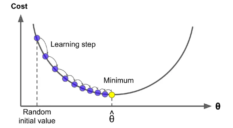
We use gradient descent to find the optimum weights.
Gradient Descent
Read more about Gradient Descent
Problem
Weights in the early layers do not touch the final output directly, where the loss/cost is calculated.
Weights are ‘buried’ behind multiple layers of non-linear transformations (like ReLU or Sigmoid).
So, how do we calculate the gradient to update the weights in first layer when the actual error information is only available at the output layer at the end.
💡 For propagating the gradient, we can use something called chain rule of differentiation.
Chain Rule
Chain rule tells us how derivatives propagate through intermediate variables.
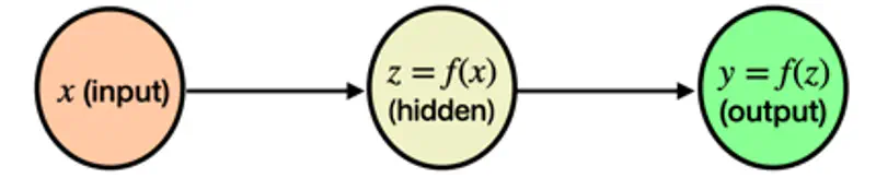
Let’s understand chain rule using a simple gear analogy.
Say we have 3 gears connected together of different radii, \(r_1\) = 1 unit, \(r_2\) = 2 units and \(r_3\) = 6 units.
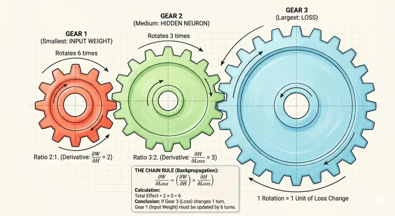
So, if the largest gear(far right) rotates 1 time, then the other smaller gears connected to it will also rotate, but since their radii is less, they will need to rotate more times to cover the same distance.
Distance covered by the largest gear in 1 rotation = \(2 \pi r_3\) = \(2 \times \pi \times 6\) = \(12 \pi\)
So, number of rotation required by middle gear \(r_2\) to cover the same distance
= \(\frac{12 \pi}{2 \pi r_2}\) = \(\frac{12 \pi}{2 \times \pi \times 2}\) = 3
Therefore, the middle gear will need to make 3 rotations if largest gear makes 1 rotation, and similarly the smallest gear(far left) will need to make 6 rotations.
So, when we see in terms of rate of change = rotations per unit time, and if we know the relation between the radii of adjacent gears, then we can propagate the rate of change from right to left.
Thus, the gradient in a deep neural network also flows back in a similar fashion from output (right) to the first layer (left).
So, we can have multiple such gears connected in a complex manner, and we just need to know the relation of a gear’s radius to the adjacent gears,
and that information is sufficient to calculate how many times that gear needs to rotate if the gear on the far right rotated once.
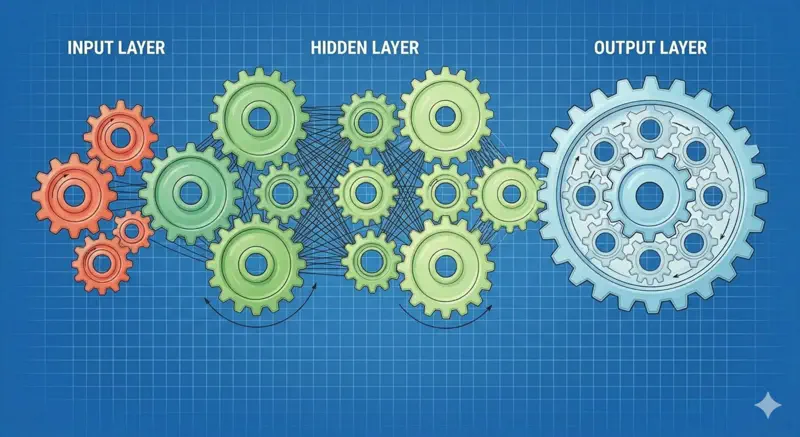
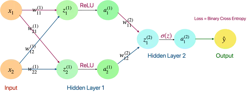
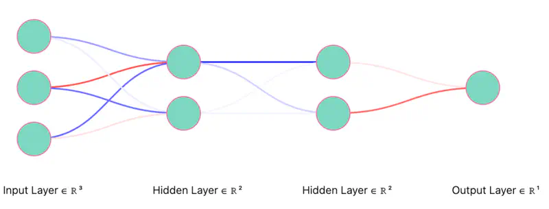
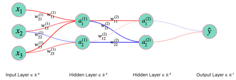
Now, lets apply this chain rule concept and understand the back propagation through a fully connected neural network.
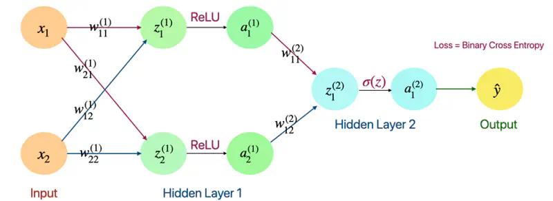
Forward Pass
Layer 1
- \(z_1^{(1)} = w_{11}^{(1)}x_1 + w_{12}^{(1)}x_2\)
- \(z_2^{(1)} = w_{21}^{(1)}x_1 + w_{22}^{(1)}x_2\)
- \(a_1^{(1)} = ReLU(z_{1}^{(1)})\)
- \(a_2^{(1)} = ReLU(z_{2}^{(1)})\)
Layer 2
- \(z_1^{(2)} = w_{11}^{(2)}a_1^{(1)} + w_{12}^{(2)}a_2^{(1)}\)
- \(a_1^{(2)} = \sigma(z_{1}^{(2)})\)
- \(\hat{y} = a_1^{(2)} = \sigma(z_{1}^{(2)})\)
Now, let’s go from right to left, calculating gradient at each point and propagating it back, using chain rule.
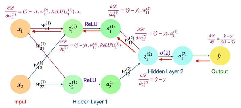
Back Propagation
Derivative of Loss w.r.t Output(\(\hat{y}\))
- Loss = Binary Cross Entropy
\[ \mathcal{L} = -[ylog(\hat{y}) + (1-y)log(1-\hat{y})] \] \[ \begin{align*} \frac{\partial{\mathcal{L}}}{\partial{\hat{y}}} &= - [\frac{y}{\hat{y}} - \frac{1-y}{1-\hat{y}}] \\ &= -[\frac{y- \cancel{y\hat{y}} -\hat{y} + \cancel{y\hat{y}}}{\hat{y}(1-\hat{y})}] \\ \therefore \frac{\partial{\mathcal{L}}}{\partial{\hat{y}}} &= \frac{\hat{y} - y}{\hat{y}(1-\hat{y})} \end{align*} \]
Derivative of Loss w.r.t \(\text{z}_1^{(2)}\)
\[ \begin{align*} \frac{\partial{\mathcal{L}}}{\partial{z_1^{(2)}}} &= \frac{\partial{\mathcal{L}}} {\partial{\hat{y}}}. \frac{\partial{\hat{y}}}{\partial{z_1^{(2)}}} \quad \text{also, } \hat{y} = a_1^{(2)} = \sigma(z_{1}^{(2)})\\ \end{align*} \]\[ \text{we know that: } \frac{\partial{\mathcal{L}}}{\partial{\hat{y}}} = \frac{\hat{y} - y}{\hat{y}(1-\hat{y})} \quad \text{so, we need to find: } \frac{\partial{\hat{y}}}{\partial{z_1^{(2)}}} = ? \]\[\text{so, } \frac{\partial{\hat{y}}}{\partial{z_1^{(2)}}} = \frac{\partial{\sigma(z_{1}^{(2)})}}{\partial{z_{1}^{(2)}}} \]\[\because \frac{\partial{\sigma(z)}}{\partial{z}} = \sigma(z).(1-\sigma(z))\]\[ \implies \frac{\partial{\hat{y}}}{\partial{z_1^{(2)}}} = \hat{y}(1-\hat{y})\]\[\frac{\partial{\mathcal{L}}}{\partial{z_1^{(2)}}} = \frac{\partial{\mathcal{L}}} {\partial{\hat{y}}}. \frac{\partial{\hat{y}}}{\partial{z_1^{(2)}}} = \frac{\hat{y} - y}{\cancel{\hat{y}(1-\hat{y})}}.\cancel{\hat{y}(1-\hat{y})}\]\[\therefore \frac{\partial{\mathcal{L}}}{\partial{z_1^{(2)}}} = \hat{y} - y\]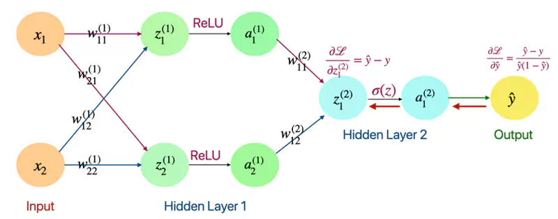
Derivative of Loss w.r.t \(\text{w}_{11}^{(2)}\) and \(a_1^{(1)}\)
\[ \begin{align*} \frac{\partial{\mathcal{L}}}{\partial{w_{11}^{(2)}}} = \frac{\partial{\mathcal{L}}}{\partial{z_1^{(2)}}}. \frac{\partial{z_1^{(2)}}}{\partial{w_{11}^{(2)}}} \end{align*} \]\[\text{we know that: } \frac{\partial{\mathcal{L}}}{\partial{z_1^{(2)}}} = \hat{y} - y \quad \text{so, we need to find: } \frac{\partial{z_1^{(2)}}}{\partial{w_{11}^{(2)}}} = ?\]\[\because z_1^{(2)} = w_{11}^{(2)}a_1^{(1)} + w_{12}^{(2)}a_2^{(1)}\]\[\implies \frac{\partial{z_1^{(2)}}}{\partial{w_{11}^{(2)}}} = a_1^{(1)} \quad \text{and } \frac{\partial{z_1^{(2)}}}{\partial{a_1^{(1)}}} = w_{11}^{(2)}\]\[ \begin{align*} \therefore \frac{\partial{\mathcal{L}}}{\partial{w_{11}^{(2)}}} = \frac{\partial{\mathcal{L}}}{\partial{z_1^{(2)}}}. \frac{\partial{z_1^{(2)}}}{\partial{w_{11}^{(2)}}} = (\hat{y} - y).a_1^{(1)} \end{align*} \]\[ \begin{align*} \text{ Similarly, } \frac{\partial{\mathcal{L}}}{\partial{a_1^{(1)}}} = \frac{\partial{\mathcal{L}}}{\partial{z_1^{(2)}}}. \frac{\partial{z_1^{(2)}}}{\partial{a_1^{(1)}}} = (\hat{y} - y).w_{11}^{(2)} \end{align*} \]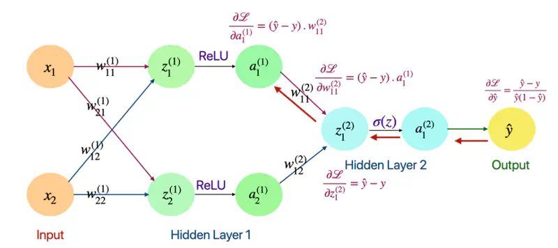
Derivative of Loss w.r.t \(\text{z}_1^{(1)}\)
\[ \begin{align*} \frac{\partial{\mathcal{L}}}{\partial{z_1^{(1)}}} = \frac{\partial{\mathcal{L}}}{\partial{a_1^{(1)}}}. \frac{\partial{a_1^{(1)}}}{\partial{z_1^{(1)}}} \end{align*} \]\[\text{we know that: } \frac{\partial{\mathcal{L}}}{\partial{a_1^{(1)}}} = (\hat{y} - y).w_{11}^{(2)} \quad \text{so, we need to find: } \frac{\partial{a_1^{(1)}}}{\partial{z_1^{(1)}}}= ?\]\[\because a_1^{(1)} = ReLU(z_{1}^{(1)})\]\[\implies \frac{\partial{a_1^{(1)}}}{\partial{z_1^{(1)}}} = \frac{\partial{ReLU(z_{1}^{(1)})}}{\partial{z_1^{(1)}}} = ReLU'(z_{1}^{(1)})\]\[ \begin{align*} \therefore \frac{\partial{\mathcal{L}}}{\partial{z_1^{(1)}}} = \frac{\partial{\mathcal{L}}}{\partial{a_1^{(1)}}}. \frac{\partial{a_1^{(1)}}}{\partial{z_1^{(1)}}} = (\hat{y} - y).w_{11}^{(2)}.ReLU'(z_{1}^{(1)}) \end{align*} \]Derivative of Loss w.r.t \(\text{w}_{11}^{(1)}\)
\[ \begin{align*} \frac{\partial{\mathcal{L}}}{\partial{w_{11}^{(1)}}} = \frac{\partial{\mathcal{L}}}{\partial{z_1^{(1)}}}. \frac{\partial{z_1^{(1)}}}{\partial{w_{11}^{(1)}}} \end{align*} \]\[\text{we know that: } \frac{\partial{\mathcal{L}}}{\partial{z_1^{(2)}}} = (\hat{y} - y).w_{11}^{(2)}.ReLU'(z_{1}^{(1)}) \quad \text{so, we need to find: } \frac{\partial{z_1^{(1)}}}{\partial{w_{11}^{(1)}}} = ?\]\[\because z_1^{(1)} = w_{11}^{(1)}x_1 + w_{12}^{(1)}x_2\]\[\implies \frac{\partial{z_1^{(1)}}}{\partial{w_{11}^{(1)}}} = x_1\]\[\therefore \frac{\partial{\mathcal{L}}}{\partial{w_{11}^{(1)}}} = \frac{\partial{\mathcal{L}}}{\partial{z_1^{(1)}}}. \frac{\partial{z_1^{(1)}}}{\partial{w_{11}^{(1)}}} = (\hat{y} - y).w_{11}^{(2)}.ReLU'(z_{1}^{(1)}).x_1\]