This is the multi-page printable view of this section. Click here to print.
Machine Learning
- 1: Introduction
- 1.1: What is ML ?
- 1.2: Types of ML
- 2: Supervised Learning
- 2.1: Linear Regression
- 2.1.1: Meaning of 'Linear'
- 2.1.2: Meaning of 'Regression'
- 2.1.3: Linear Regression
- 2.1.4: Probabilistic Interpretation
- 2.1.5: Convex Function
- 2.1.6: Gradient Descent
- 2.1.7: Polynomial Regression
- 2.1.8: Data Splitting
- 2.1.9: Cross Validation
- 2.1.10: Bias Variance Tradeoff
- 2.1.11: Regularization
- 2.1.12: Regression Metrics
- 2.1.13: Assumptions
- 2.2: Logistic Regression
- 2.2.1: Binary Classification
- 2.2.2: Log Loss
- 2.2.3: Regularization
- 2.2.4: Log Odds
- 2.2.5: Probabilistic Interpretation
- 2.3: K Nearest Neighbors
- 2.3.1: KNN Introduction
- 2.3.2: KNN Optimizations
- 2.3.3: Curse Of Dimensionality
- 2.3.4: Bias Variance Tradeoff
- 2.4: Decision Tree
- 2.4.1: Decision Trees Introduction
- 2.4.2: Purity Metrics
- 2.4.3: Decision Trees For Regression
- 2.4.4: Regularization
- 2.4.5: Bagging
- 2.4.6: Random Forest
- 2.4.7: Extra Trees
- 2.4.8: Boosting
- 2.4.9: AdaBoost
- 2.4.10: Gradient Boosting Machine
- 2.4.11: GBDT Algorithm
- 2.4.12: GBDT Example
- 2.4.13: Advanced GBDT Algorithms
- 2.4.14: XgBoost
- 2.4.15: LightGBM
- 2.4.16: CatBoost
- 2.5: Support Vector Machine
- 2.5.1: SVM Intro
- 2.5.2: Hard Margin SVM
- 2.5.3: Soft Margin SVM
- 2.5.4: Primal Dual Equivalence
- 2.5.5: Kernel Trick
- 2.5.6: RBF Kernel
- 2.5.7: Support Vector Regression
- 2.6: Naive Bayes'
- 2.6.1: Naive Bayes Intro
- 2.6.2: Naive Bayes Issues
- 2.6.3: Naive Bayes Example
- 3: Unsupervised Learning
- 3.1: K Means
- 3.1.1: K Means
- 3.1.2: Lloyds Algorithm
- 3.1.3: K Means++
- 3.1.4: K Medoid
- 3.1.5: Clustering Quality Metrics
- 3.1.6: Silhouette Score
- 3.2: Hierarchical Clustering
- 3.2.1: Hierarchical Clustering
- 3.3: DBSCAN
- 3.3.1: DBSCAN
- 3.4: Gaussian Mixture Model
- 3.4.1: Gaussian Mixture Models
- 3.4.2: Latent Variable Model
- 3.4.3: Expectation Maximization
- 3.5: Anomaly Detection
- 3.5.1: Anomaly Detection
- 3.5.2: Elliptic Envelope
- 3.5.3: One Class SVM
- 3.5.4: Local Outlier Factor
- 3.5.5: Isolation Forest
- 3.5.6: RANSAC
- 3.6: Dimensionality Reduction
- 4: Feature Engineering
- 4.1: Data Pre Processing
- 4.2: Categorical Variables
- 4.3: Feature Engineering
- 4.4: Data Leakage
- 4.5: Model Interpretability
- 5: ML System
- 6: Interview Questions
1 - Introduction
1.1 - What is ML ?
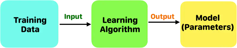
The machine learning lifecycle ♼ is generally divided into two main stages:
- Training Phase
- Runtime (Inference) Phase
Training Phase:
Where the machine learning model is developed and taught to understand a specific task using a large volume
of historical data.
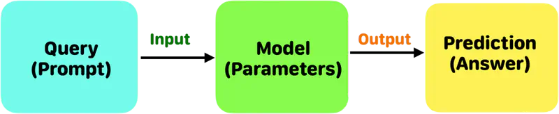
Runtime (Inference) Phase:
Where the fully trained and deployed model is put to practical use in a real-world 🌎 environment, i.e.,
to make predictions on new, unseen data.
End of Section
1.2 - Types of ML
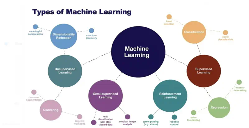
Supervised Learning uses labelled data (input-output pairs) to predict outcomes, such as, spam filters.
- Regression
- Classification
Unsupervised Learning finds hidden patterns in unlabelled data (like customer segmentation).
- Clustering (k-means, hierarchical)
- Dimensionality Reduction and Data Visualization (PCA, t-SNE, UMAP)
Semi-Supervised Learning uses a mix of both, leveraging a small amount of labelled data with a large amount of
unlabelled data to improve accuracy.
- Pseudo-labeling
- Graph-based methods
1. Pseudo-labelling:
- A model is initially trained on the available, limited labelled dataset.
- This trained model is then used to predict labels for the unlabelled data.These predictions are called ‘pseudo-labels’.
- The model is then retrained using both the original labelled data and the newly pseudo-labelled data.
Benefit:
It effectively expands the training data by assigning labels to previously unlabelled examples,
allowing the model to learn from a larger dataset.
2. Graph-based methods:
- Data points (both labelled and unlabelled) are represented as nodes in a graph.
- Edges are established between nodes based on their similarity or proximity in the feature space.The weight of an edge often reflects the degree of similarity.
- The core principle is that similar data points should have similar labels.This assumption is propagated through the graph, effectively ‘spreading’ the labels from the labelled nodes to the unlabelled nodes based on the graph structure.
- Various algorithms, such as label propagation or graph neural networks (GNNs), can be employed to infer the labels of unlabelled nodes.
Benefit:
These methods are particularly useful when the data naturally exhibits a graph-like structure or when local
neighborhood information is crucial for classification.
Agent learns to make optimal decisions by interacting with an environment, receiving rewards (positive feedback)
or penalties (negative feedback) for its actions.
- Mimic human trial-and-error learning to achieve a goal 🎯.
- Agent: The learning entity that makes decisions and takes actions within the environment.
- Environment: The external system with which the agent interacts.It defines the rules, states, and the consequences of the agent’s actions.
- State: A specific configuration or situation of the environment at a given point in time.
- Action: A move or decision made by the agent in a particular state.
- Reward: A numerical signal received by the agent from the environment, indicating the desirability of an action taken
in a specific state.
Positive rewards encourage certain behaviors, while negative rewards (penalties) discourage them. - Policy: The strategy or mapping that defines which action the agent should take in each state to maximize long-term rewards 💰.
- Exploration: The agent tries out new actions to discover their effects and potentially find better strategies.
- Exploitation: The agent utilizes its learned knowledge to choose actions that have yielded high rewards in the past.
Note: The agent continuously balances exploration and exploitation to refine its policy and achieve the optimal behavior.
Large Language Models (LLMs) are deep learning models that often employ unsupervised learning techniques during their pre-training phase.
LLMs are trained on massive amounts of raw, unlabelled text data (e.g., books, articles, web pages) to predict the next
word in a sequence or fill in masked words.
This process, often called self-supervised learning, allows the model to learn grammar, syntax, semantics,
and general world knowledge by identifying statistical relationships within the text.
LLMs generally also undergo supervised fine-tuning (SFT) for specific tasks, where they are trained on labeled datasets to improve performance on those tasks.
Reinforcement Learning from Human Feedback (RLHF) allows LLMs to learn from human judgment, enabling them to generate more nuanced, context-aware, and ethically aligned outputs that better meet human expectations.
End of Section
2.1.1 - Meaning of 'Linear'
Equation of a line is of the form \(y = mx + c\).
To represent a line in 2D space, we need 2 things:
- m = slope or direction of the line
- c = y-intercept or distance from the origin
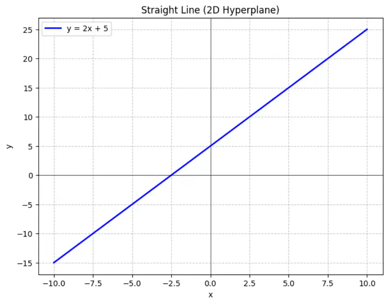
Similarly,
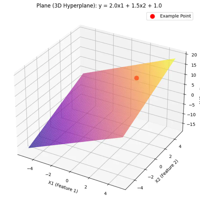
A hyperplane is a lower (d-1) dimensional sub-space that divides a d-dimensional space into 2 distinct parts.
Equation of a hyperplane:
Here, ‘y’ is expressed as a linear combination of parameters - \( w_0, w_1, w_2, \dots, w_n \)
Hence - Linear means the model is ‘linear’ with respect to its parameters NOT the variables.
Read more about Hyperplane
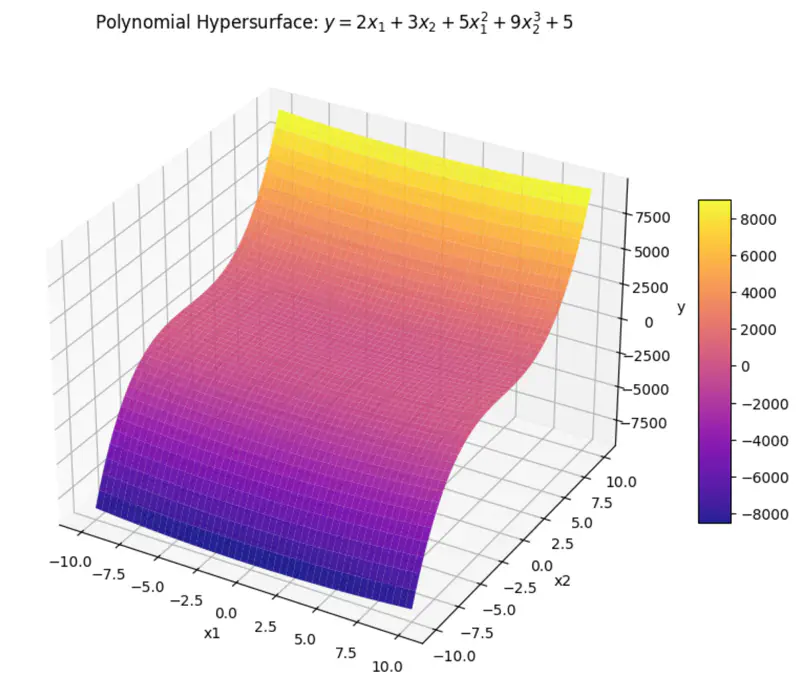
can be rewritten as:
\[y = w_1x_1 + w_2x_2 + w_3x_3 + w_4x_4 + w_0\]where, \(x_3 = x_1^2 ~ and ~ x_4 = x_2^3 \)
\(x_3 ~ and ~ x_4 \) are just 2 new (polynomial) variables.
And, ‘y’ is still a linear combination of parameters: \(w_0, w_1, \dots w_4\)
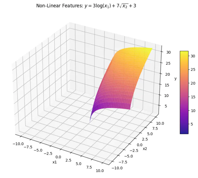
can be rewritten as:
\[y = w_1x_1 + w_2x_2 + w_0\]where, \(x_1 = log(x) ~ and ~ x_2 = \sqrt{x} \)
\(x_1 ~ and ~ x_2 \) are are transformations of variable \(x\).
And, ‘y’ is still a linear combination of parameters: \(w_0, w_1, ~and~ w_2\)
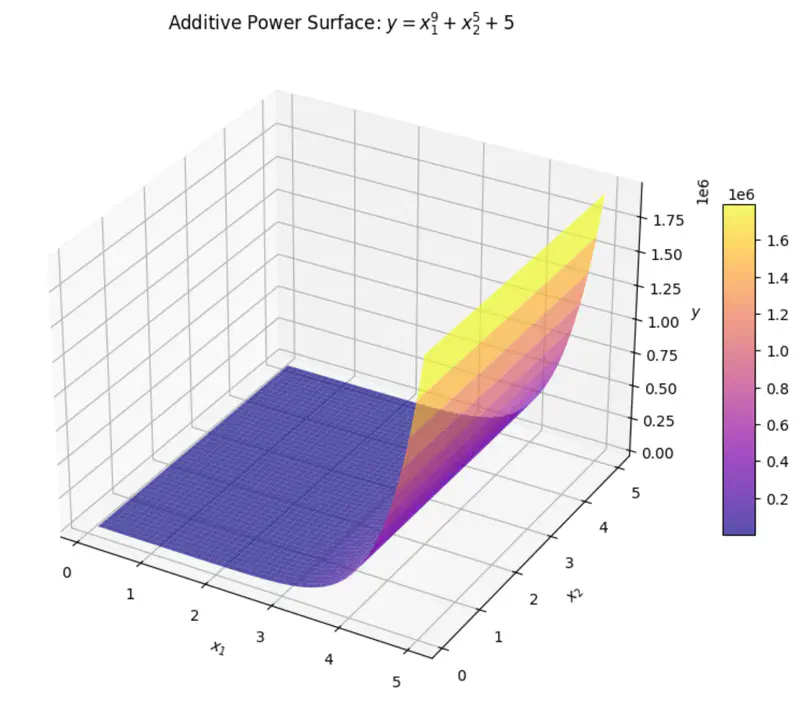
Even if we take log, we get:
\[log(y) = w_1log(x_1) + w_2log(x_2) + log(w_0)\]here, \(log(w_0) \) parameter is NOT linear.
End of Section
2.1.2 - Meaning of 'Regression'
Regression = Going Back
Regression has a very specific historical origin that is different from its current statistical meaning.
Sir Francis Galton (19th century), cousin of Charles Darwin, coined 🪙 this term.
Observation:
Galton observed that -
the children 👶 of unusually tall ⬆️ parents 🧑🧑🧒🧒,
tended to be shorter ⬇️ than their parents 🧑🧑🧒🧒,
and children 👶 of unusually short ⬇️ parents 🧑🧑🧒🧒,
tended to be taller ⬆️ than their parents 🧑🧑🧒🧒.
Galton named this biological tendency - ‘regression towards mediocrity/mean’.
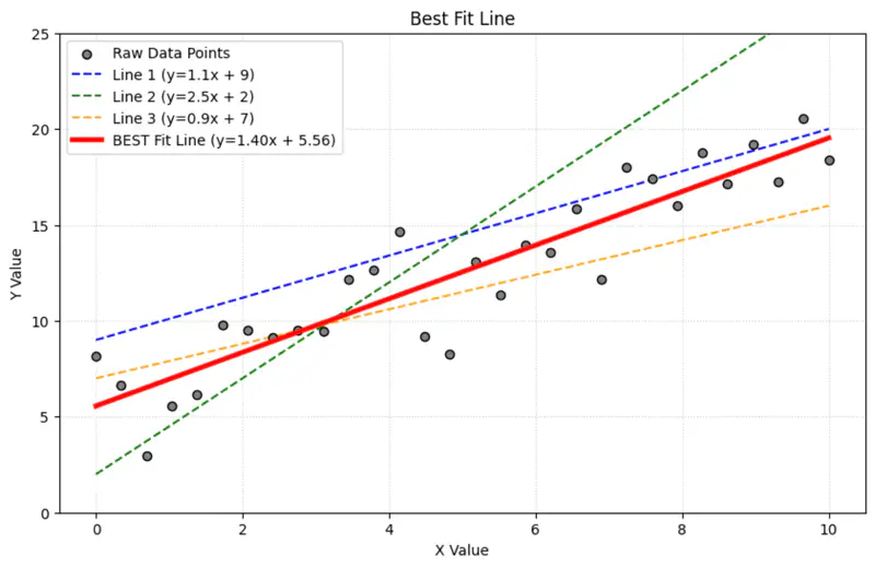
Galton used method of least squares to model this relationship, by fitting a line to the data 📊.
Regression = Fitting a Line
Over time ⏳, the name ‘regression’ got permanently attached to the method of fitting line to the data 📊.
Today in statistics and machine learning, ‘regression’ universally refers to the method of finding the
‘line of best fit’ for a set of data points, NOT the concept of ‘regressing towards the mean’.
End of Section
2.1.3 - Linear Regression
Let’s understand linear regression using an example to predict salary.
Predict the salary 💰 of an IT employee, based on various factors, such as, years of experience, domain, role, etc.
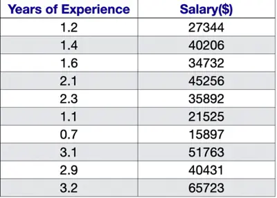
Let’s start with a simple problem and predict the salary using only one input feature.
Goal 🎯 : Find the line of best fit.
Plot: Salary vs Years of Experience
\[y = mx + c = w_1x + w_0\]Slope = \(m = w_1 \)
Intercept = \(c = w_0\)
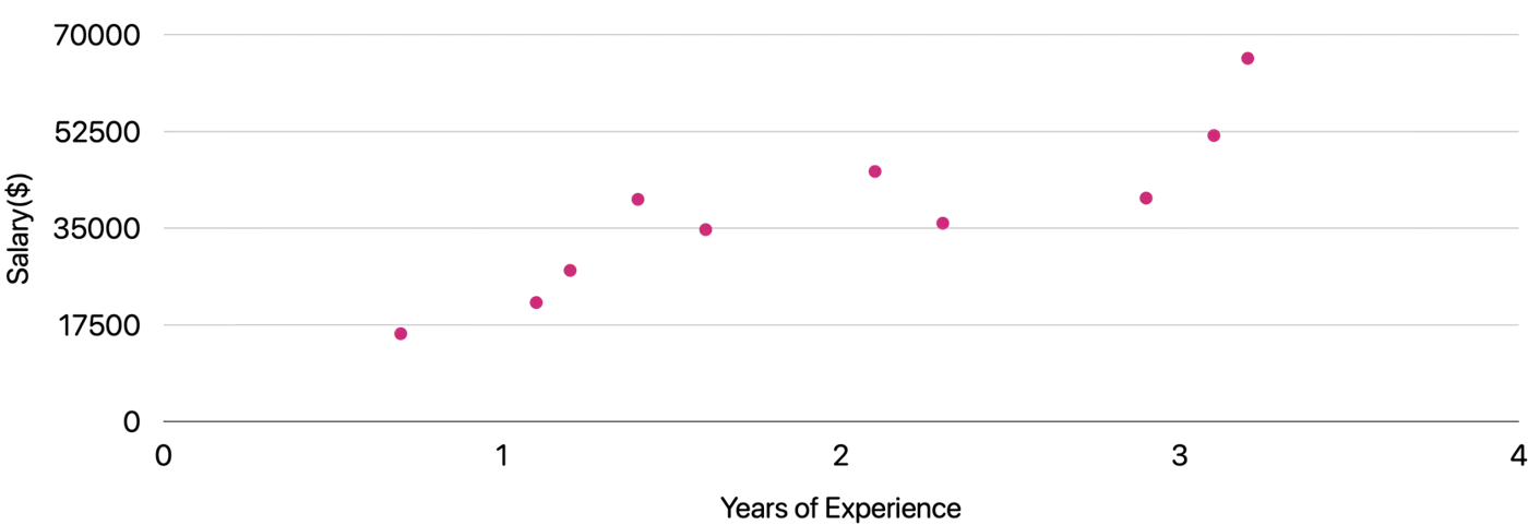
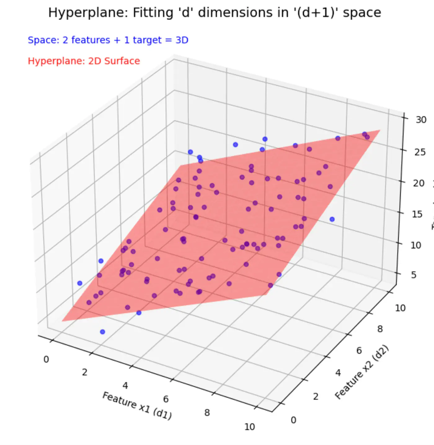
Similarly, if we include other factors/features impacting the salary 💰, such as, domain, role, etc, we get an equation of a fitting hyperplane:
\[y = w_1x_1 + w_2x_2 + \dots + w_dx_d + w_0\]where,
\[ \begin{align*} x_1 &= \text{Years of Experience} \\ x_2 &= \text{Domain (Tech, BFSI, Telecom, etc.)} \\ x_3 &= \text{Role (Dev, Tester, DevOps, ML, etc.)} \\ x_d &= d^{th} ~ feature \\ w_0 &= \text{Salary of 0 years experience} \\ \end{align*} \]Space = ’d’ features + 1 target variable = ’d+1’ dimensions
In a ’d+1’ dimensional space, we try to fit a ’d’ dimensional hyperplane.
Let, data = \( {(x_i, y_i)}_{i=1}^N ; ~ x_i \in R^d , y_i \in R^d\)
where, N = number of training samples.
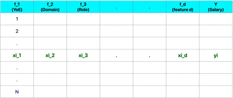
Note: Fitting hyperplane (\(y = w_1x_1 + w_2x_2 + \dots + w_dx_d + w_0\)) is the model.
Objective 🎯: find the parameters/weights (\(w_0, w_1, w_2, \dots w_d \)) of the model.
\(\mathbf{w} = \begin{bmatrix} w_1 \\ w_2 \\ \vdots \\ w_d \end{bmatrix}_{\text{d x 1}}\)
\( \mathbf{x_i} = \begin{bmatrix} x_{i_1} \\ x_{i_2} \\ \vdots \\ x_{i_d} \end{bmatrix}_{\text{d x 1}} \)
\( \mathbf{y} = \begin{bmatrix} y_1 \\ y_2 \\ \vdots \\ y_i \\ \vdots \\ y_n \end{bmatrix}_{\text{n x 1}} \)
\( X =
\begin{bmatrix}
x_{11} & x_{12} & \cdots & x_{1d} \\
x_{21} & x_{22} & \cdots & x_{2d} \\
\vdots & \vdots & \ddots & \vdots \\
x_{i1} & x_{i2} & \cdots & x_{id} \\
\vdots & \vdots & \ddots & \vdots \\
x_{n1} & x_{n2} & \cdots & x_{nd} \\
\end{bmatrix}
_{\text{n x d}}
\)
Prediction:
Error = Actual - Predicted
\[ \epsilon_i = y_i - \hat{y_i}\]Goal 🎯: Minimize error between actual and predicted.
We can quantify the error for a single data point in following ways:
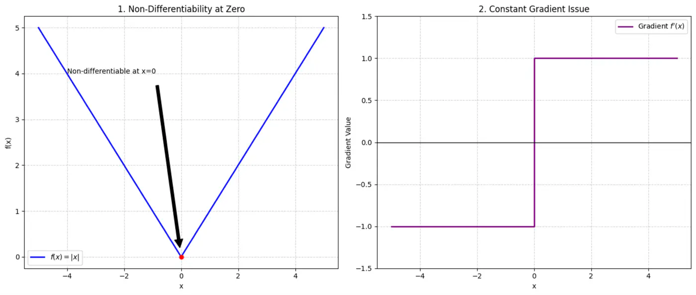
- Absolute error = \(|y_i - \hat{y_i}|\)
- Squared error = \((y_i - \hat{y_i})^2\)
Not differentiable at x=0, required for gradient descent.
Constant gradient, i.e \(\pm 1\), model learns at same rate, whether the error is large or small.
Average loss across all data points.
Mean Squared Error (MSE) =
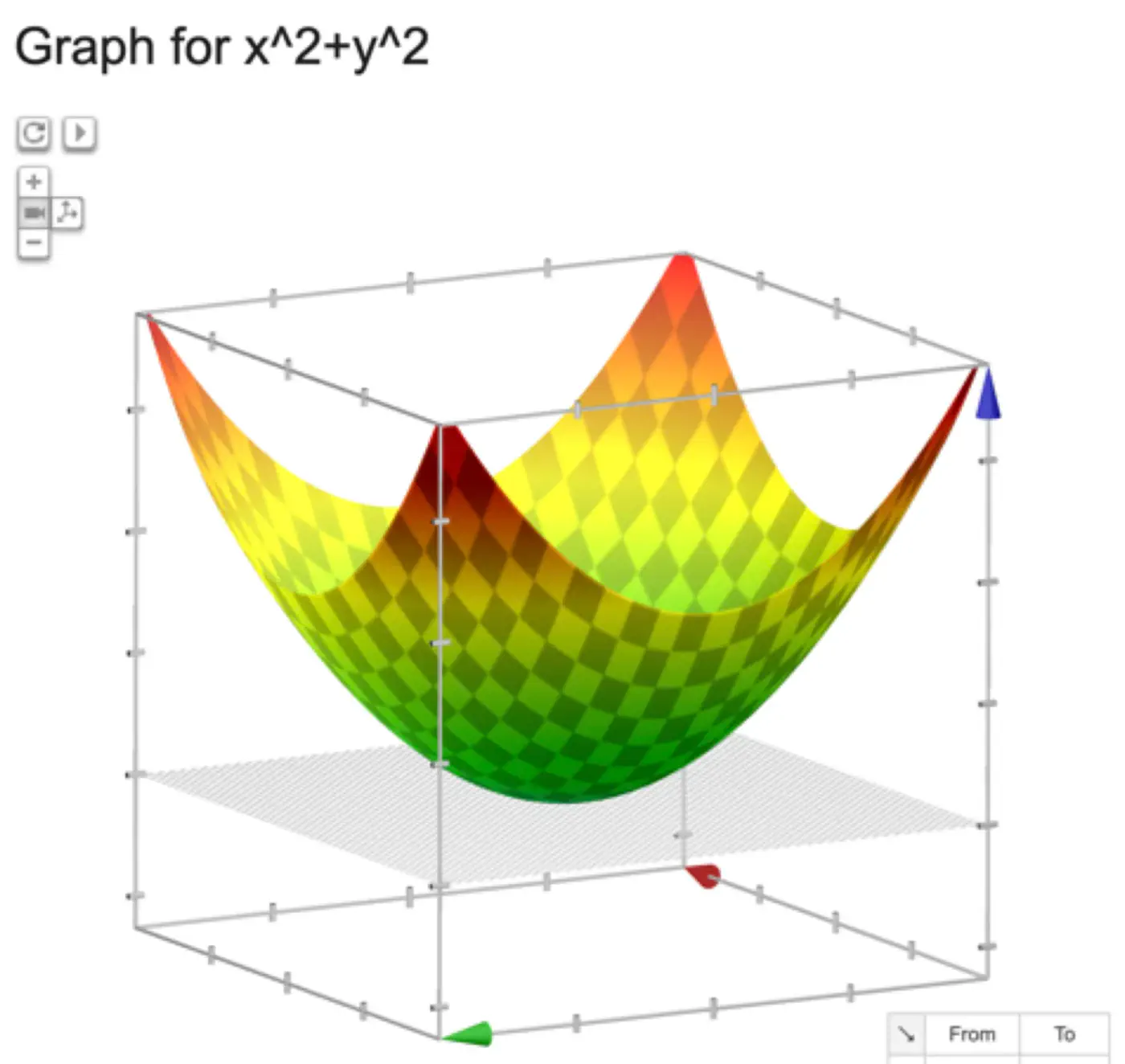
\[ J(w) = \frac{1}{n} \sum_{i=1}^N (y_i - \hat{y_i})^2 \]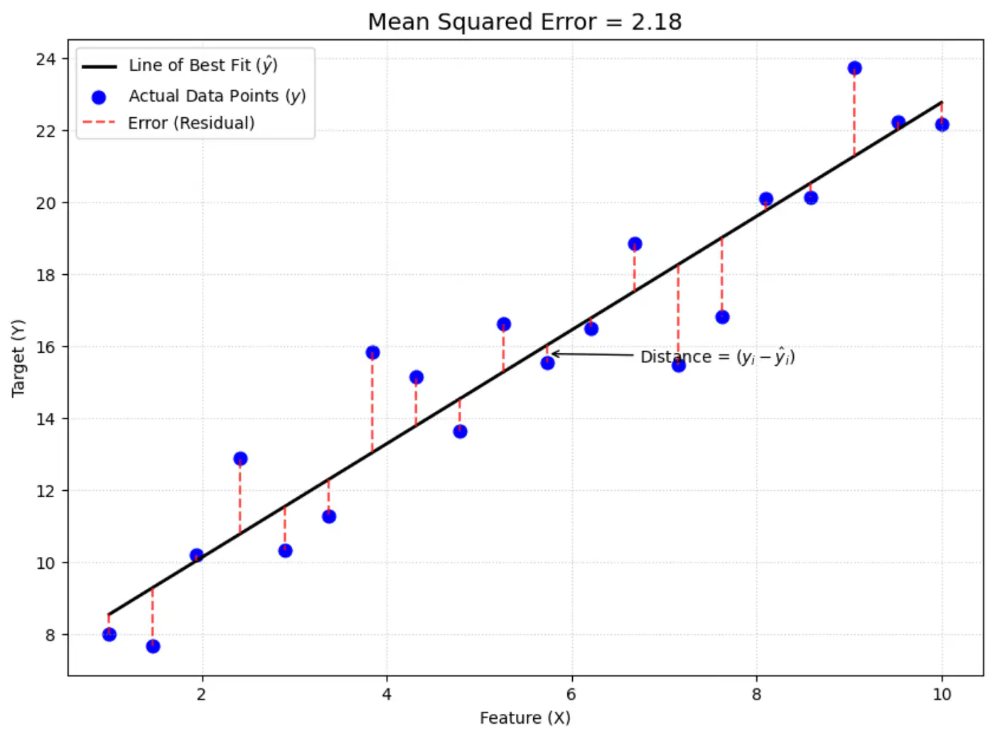
The above equation is quadratic in \(w_0, w_1, w_2, \dots w_d \).
Below is an image of a Paraboloid in 3D, similarly we will have a Paraboloid in ’d’ dimensions.
In order to find the minima of the cost function we need to take its derivative w.r.t weights and equate to 0.
\[ \begin{align*} \frac{\partial{J(w)}}{\partial{w_0}} = 0 \\ \frac{\partial{J(w)}}{\partial{w_1}} = 0 \\ \frac{\partial{J(w)}}{\partial{w_2}} = 0 \\ \vdots \\ \frac{\partial{J(w)}}{\partial{w_d}} = 0 \\ \end{align*} \]We have ‘d+1’ linear equations to solve for ‘d+1’ weights \(w_0, w_1, w_2, \dots , w_d\).
But solving ‘d+1’ system of linear equations (called the ’normal equations’) is tedious and NOT used for practical purposes.
where,
\(\mathbf{w} = \begin{bmatrix} w_1 \\ w_2 \\ \vdots \\ w_d \end{bmatrix}_{\text{d x 1}}\)
\( \mathbf{x_i} = \begin{bmatrix} x_{i_1} \\ x_{i_2} \\ \vdots \\ x_{i_d} \end{bmatrix}_{\text{d x 1}} \)
\( \mathbf{y} = \begin{bmatrix} y_1 \\ y_2 \\ \vdots \\ y_i \\ \vdots \\ y_n \end{bmatrix}_{\text{n x 1}} \)
\( X =
\begin{bmatrix}
x_{11} & x_{12} & \cdots & x_{1d} \\
x_{21} & x_{22} & \cdots & x_{2d} \\
\vdots & \vdots & \ddots & \vdots \\
x_{i1} & x_{i2} & \cdots & x_{id} \\
\vdots & \vdots & \ddots & \vdots \\
x_{n1} & x_{n2} & \cdots & x_{nd} \\
\end{bmatrix}
_{\text{n x d}}
\)
Prediction:
Let’s expand the cost function J(w):
\[ \begin{align*} J(w) &= \frac{1}{n} (y - Xw)^2 \\ &= \frac{1}{n} (y - Xw)^T(y - Xw) \\ &= \frac{1}{n} (y^T - w^TX^T)(y - Xw) \\ J(w) &= \frac{1}{n} (y^Ty - w^TX^Ty - y^TXw + w^TX^TXw) \end{align*} \]Since,\(w^TX^Ty\), is a scalar, so it is equal to its transpose.
\[ w^TX^Ty = (w^TX^Ty)^T = y^TXw\]\[ J(w) = \frac{1}{n} (y^Ty - y^TXw - y^TXw + w^TX^TXw)\]\[ J(w) = \frac{1}{n} (y^Ty - 2y^TXw + w^TX^TXw) \]Note: \(X^2 = X^TX\) and \((AB)^T = B^TA^T\)
To find the minimum, take the derivative of cost function J(w) w.r.t ‘w’, and equate to 0 vector.
\[\frac{\partial{J(w)}}{\partial{w}} = \vec{0}\]\[ \begin{align*} &\frac{\partial{[\frac{1}{n} (y^Ty - 2y^TXw + w^TX^TXw)]}}{\partial{w}} = 0\\ & \implies 0 - 2X^Ty + (X^TX + X^TX)w = 0 \\ & \implies \cancel{2}X^TXw = \cancel{2} X^Ty \\ & \therefore \mathbf{w} = (X^TX)^{-1}X^T\mathbf{y} \end{align*} \]Note: \(\frac{\partial{(a^T\mathbf{x})}}{\partial{\mathbf{x}}} = a\) and \(\frac{\partial{(\mathbf{x}^TA\mathbf{x})}}{\partial{\mathbf{x}}} = (A + A^T)\mathbf{x}\)
This is the closed-form solution of normal equations.
- Inverse may NOT exist (non-invertible).
- Time complexity of calculating the inverse is O(n^3).
If the inverse does NOT exist then we can use the approximation of the inverse, also called Pseudo Inverse or Moore Penrose Inverse (\(A^+\)).
Moore Penrose Inverse ( \(A^+\)) is calculated using Singular Value Decomposition (SVD).
SVD of \(A = U \Sigma V^T\)
Pseudo Inverse \(A^+ = V \Sigma^+ U^T\)
Where, \(\Sigma^+\) is a transpose of \(\Sigma\) with reciprocals of non-zero singular values on its diagonals.
e.g:
Note: Time Complexity = O(mn^2)
End of Section
2.1.4 - Probabilistic Interpretation
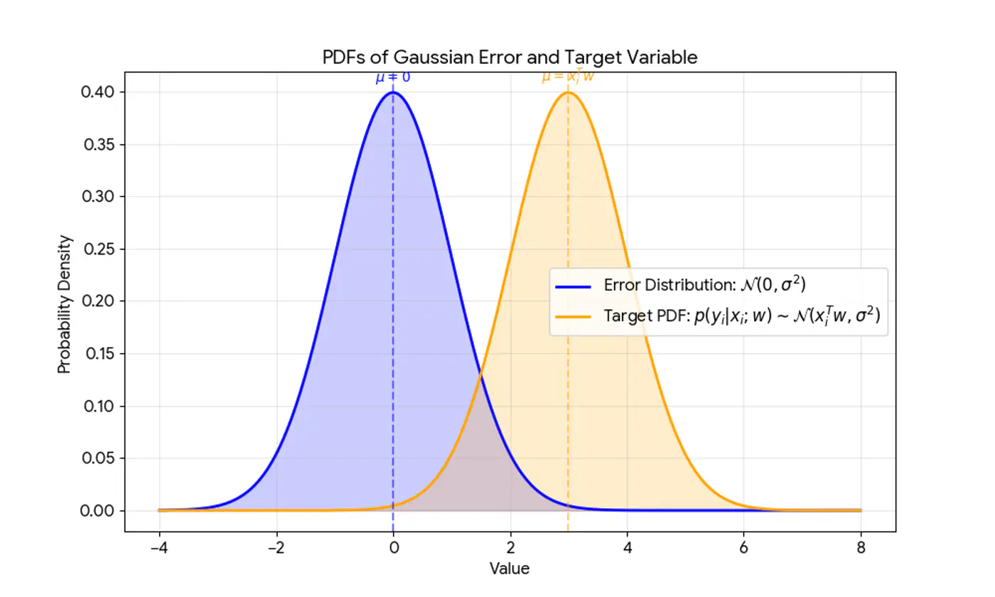
Error = Random Noise, Un-modeled effects
\[ \begin{align*} \epsilon_i = y_i - \hat{y_i} \\ \implies y_i = \hat{y_i} + \epsilon_i \\ \because \hat{y_i} = x_i^Tw \\ \therefore y_i = x_i^Tw + \epsilon_i \\ \end{align*} \]Actual value(\(y_i\)) = Deterministic linear predictor(\(x_i^Tw\)) + Error term(\(\epsilon_i\))
- Independent and Identically Distributed (I.I.D):
Each error term is independent of others. - Normal (Gaussian) Distributed:
Error follows a normal distribution with mean = 0 and a constant variance, .
This implies that the target variable itself is a random variable, normally distributed around the linear relationship.
\[(y_{i}|x_{i};w)∼N(x_{i}^{T}w,\sigma^{2})\]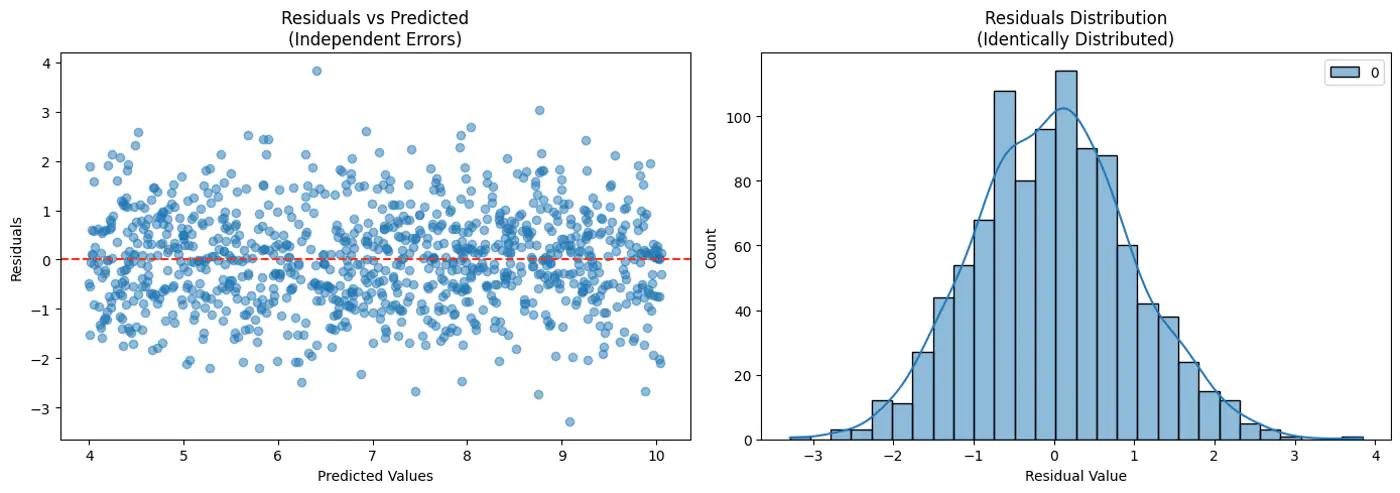
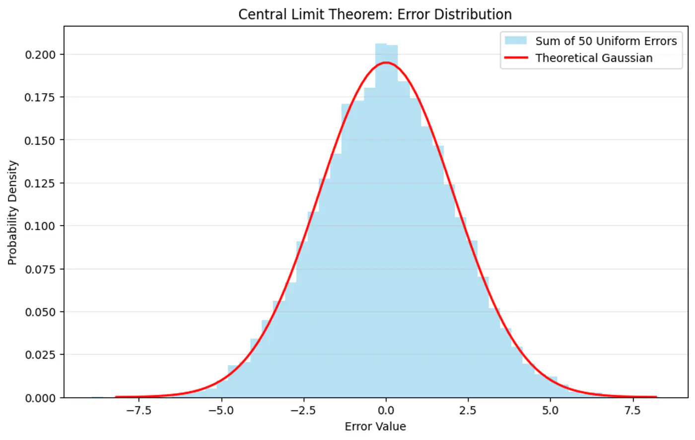
Central Limit Theorem (CLT) states that for a sequence of I.I.D random variables, the distribution of the sample mean(sum) approximates to a normal distribution, regardless of the original population distribution.
- Probability (Forward View):
Quantifies the chance of observing a specific outcome given a known, fixed model. - Likelihood (Backward/Inverse View):
Inverse concept used for inference (working backward from results to causes). It is a function of the parameters and measures how ‘likely’ a specific set of parameters makes the observed data appear.
‘Find the most plausible explanation for what I see.'
The goal of the probabilistic interpretation is to find the parameters ‘w’ that maximize the probability (likelihood) of observing the given dataset.
Assumption: Training data is I.I.D.
\[ \begin{align*} Likelihood &= \mathcal{L}(w) \\ \mathcal{L}(w) &= p(y|x;w) \\ &= \prod_{i=1}^N p(y_i| x_i; w) \\ &= \prod_{i=1}^N \frac{1}{\sigma\sqrt{2\pi}}e^{-\frac{(y_i-x_i^Tw)^2}{2\sigma^2}} \end{align*} \]Maximizing the likelihood function is mathematically complex due to the product term and the exponential function.
A common simplification is to maximize the log-likelihood function instead, which converts the product into a sum.
Note: Log is a strictly monotonically increasing function.
Note: The first term is constant w.r.t ‘w'.
So, we need to find parameters ‘w’ that maximize the log likelihood.
\[ \begin{align*} log \mathcal{L}(w) & \propto -\frac{1}{2\sigma^2} \sum_{i=1}^N (y_i-x_i^Tw)^2 \\ & \because \frac{1}{2\sigma^2} \text{ is constant} \\ log \mathcal{L}(w) & \propto -\sum_{i=1}^N (y_i-x_i^Tw)^2 \\ \end{align*} \]Maximizing the log-likelihood is equivalent to minimizing the sum of squared errors, which is the exact objective of the ordinary least squares (OLS) method.
\[ \underset{w}{\mathrm{min}}\ J(w) = \underset{w}{\mathrm{min}}\ \sum_{i=1}^N (y_i - x_i^Tw)^2 \]End of Section
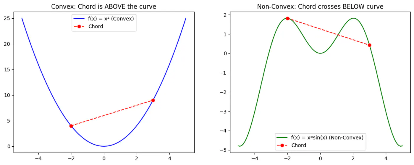
2.1.5 - Convex Function
Refers to a property of a function where a line segment connecting any two points on its graph lies above or on the graph itself.
A convex function is curved upwards.
MSE cost function J(w) is convex because its Hessian (H) is always positive semi definite.
\[\nabla J(\mathbf{w})=\frac{1}{n}\mathbf{X}^{T}(\mathbf{Xw}-\mathbf{y})\]\[\mathbf{H}=\frac{\partial (\nabla J(\mathbf{w}))}{\partial \mathbf{w}^{T}}=\frac{1}{n}\mathbf{X}^{T}\mathbf{X}\]\[\therefore \mathbf{H} = \nabla^2J(w) = \frac{1}{n} \mathbf{X}^{T}\mathbf{X}\]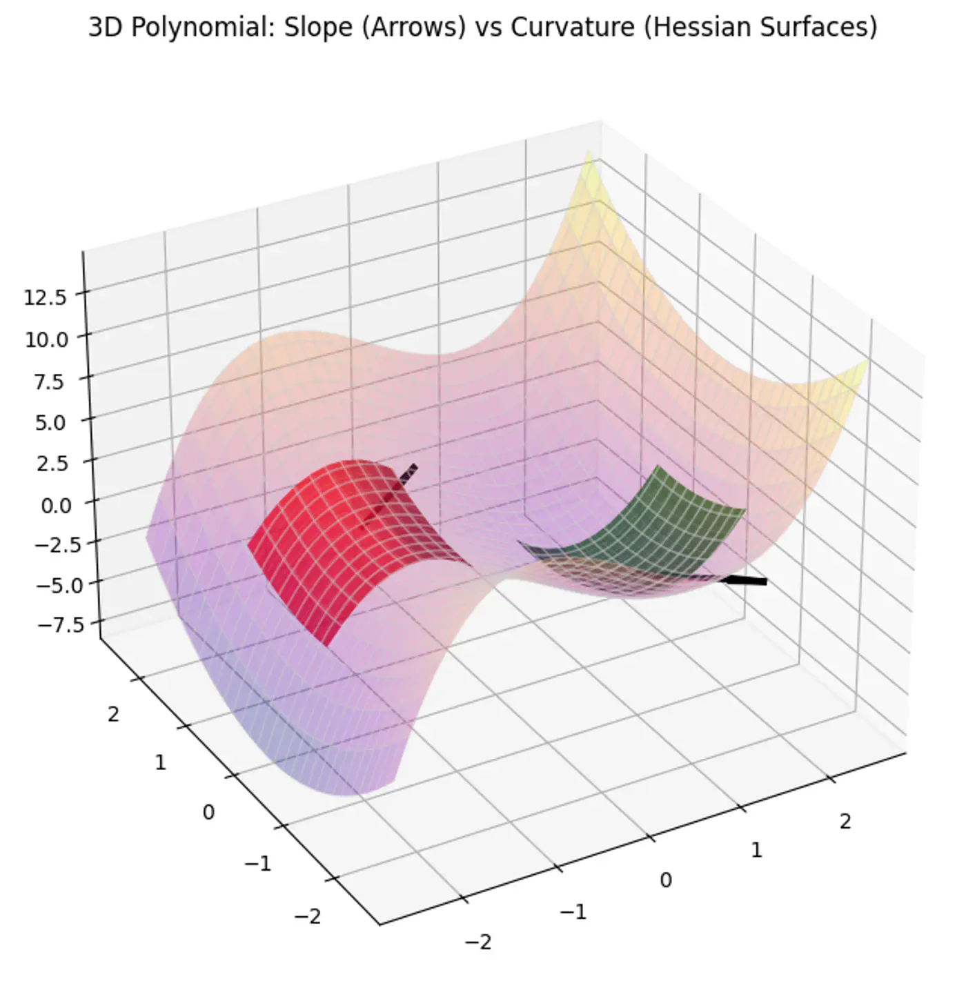
A matrix H is positive semi-definite if and only if for any non-zero vector ‘z’, the quadratic form \(z^THz \ge 0\).
For the Hessian of J(w),
\[ z^THz = z^T(\frac{1}{n}X^TX)z = \frac{1}{n}(Xz)^T(Xz) \]\((Xz)^T(Xz) = \lVert Xz \rVert^2\) = squared L2 norm (magnitude) of the vector
Note: The squared norm of any real-valued vector is always \(\ge 0\).
End of Section
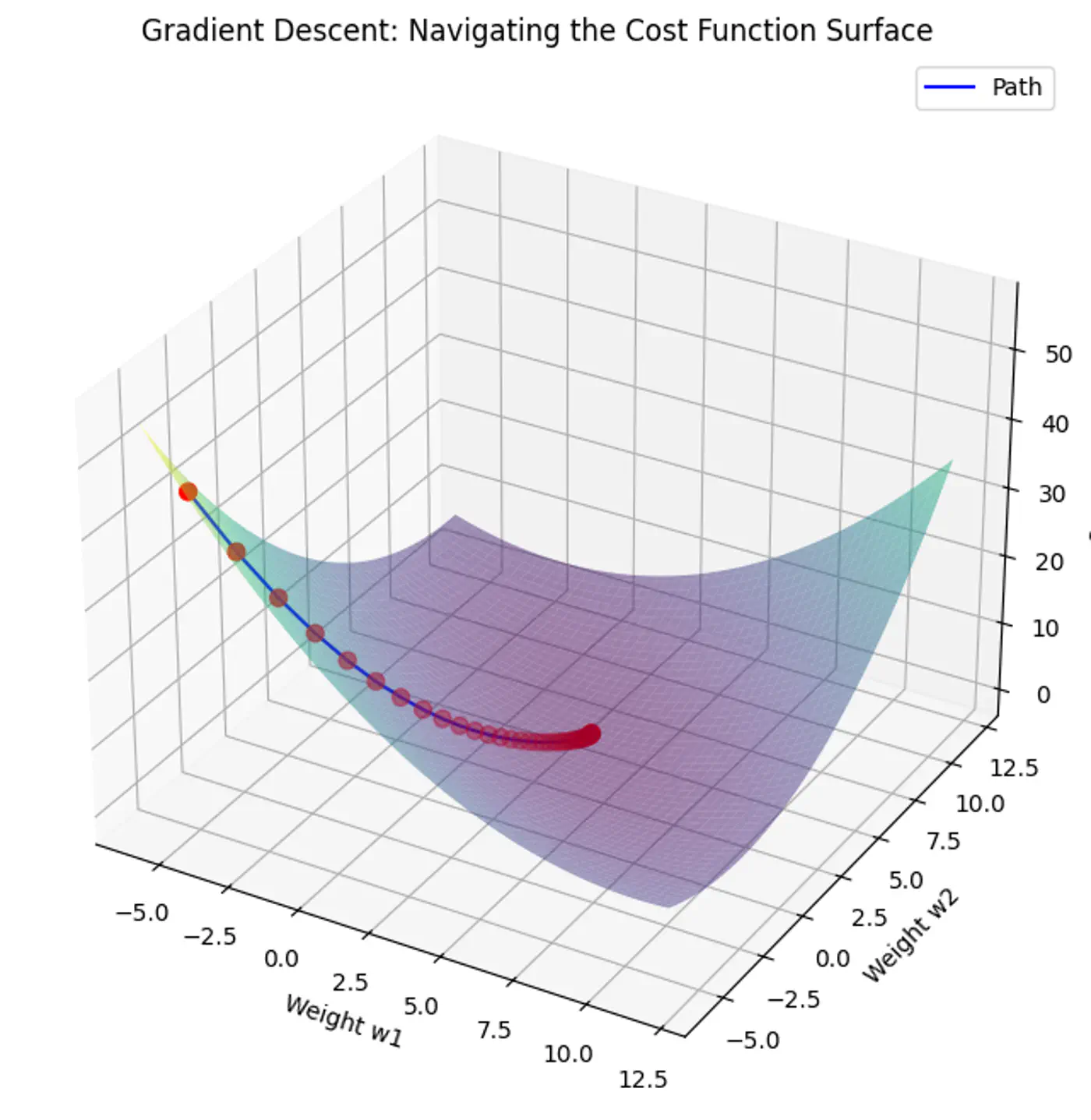
2.1.6 - Gradient Descent
Minimize the cost 💰function.
\[J(w)=\frac{1}{2n}(y-Xw)^{2}\]Note: The 1/2 term is included simply to make the derivative cleaner (it cancels out the 2 from the square).
Normal Equation (Closed-form solution) jumps straight to the optimal point in one step.
\[w=(X^{T}X)^{-1}X^{T}y\]But it is not always feasible and computationally expensive 💰(due to inverse calculation 🧮)
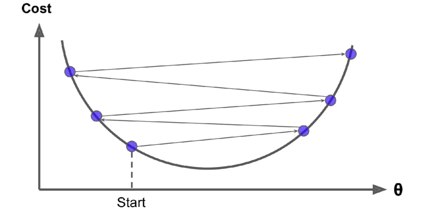
An iterative optimization algorithm slowly nudges parameters ‘w’ towards a value that minimize the cost💰 function.
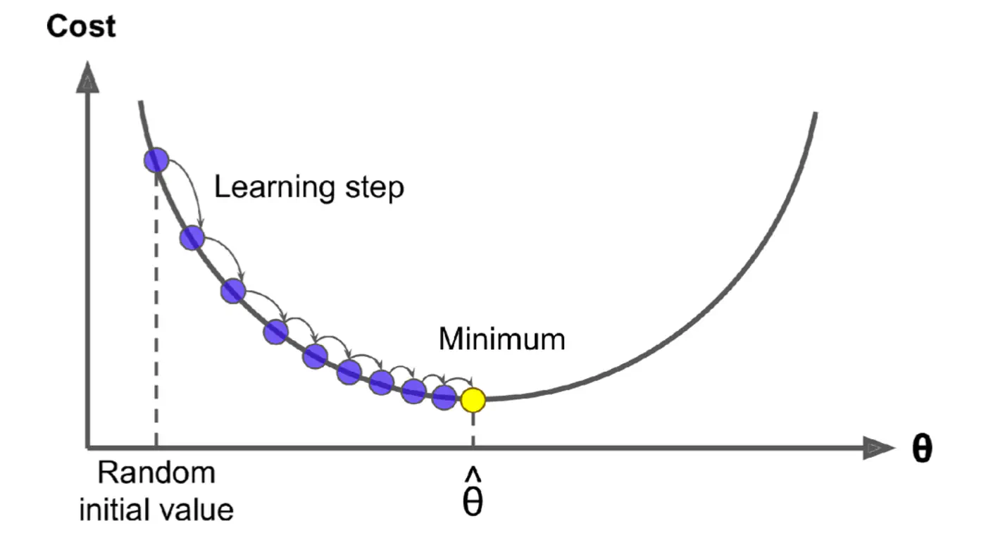
- Initialize the weights/parameters with random values.
- Calculate the gradient of the cost function at current parameter values.
- Update the parameters using the gradient. \[ w_{new} = w_{old} - \eta \frac{\partial{J(w)}}{\partial{w_{old}}} \] \( \eta \) = learning rate or step size to take for each parameter update.
- Repeat 🔁 steps 2 and 3 iteratively until convergence (to minima).
Applying chain rule:
\[ \begin{align*} &\text{Let } u = (y - Xw) \\ &\text{Derivative of } u^2 \text{ w.r.t 'w' }= 2u.\frac{\partial{u}}{\partial{w}} \\ \frac{\partial{(\frac{1}{2n} (y - Xw)^2)}}{\partial{w}} &= \frac{1}{\cancel2n}.\cancel2(y - Xw).\frac{\partial{(y - Xw)}}{\partial{w}} \\ &= \frac{1}{n}(y - Xw).X^T.(-1) \\ \therefore \frac{\partial{J(w)}}{\partial{w}} &= \frac{1}{n}X^T(Xw - y) \end{align*} \]Note: \(\frac{∂(a^{T}x)}{∂x}=a\)
Update parameter using gradient:
\[ w_{new} = w_{old} - \eta'. X^T(Xw - y) \]- Most important hyper parameter of gradient descent.
- Dictates the size of the steps taken down the cost function surface.
Small \(\eta\) ->
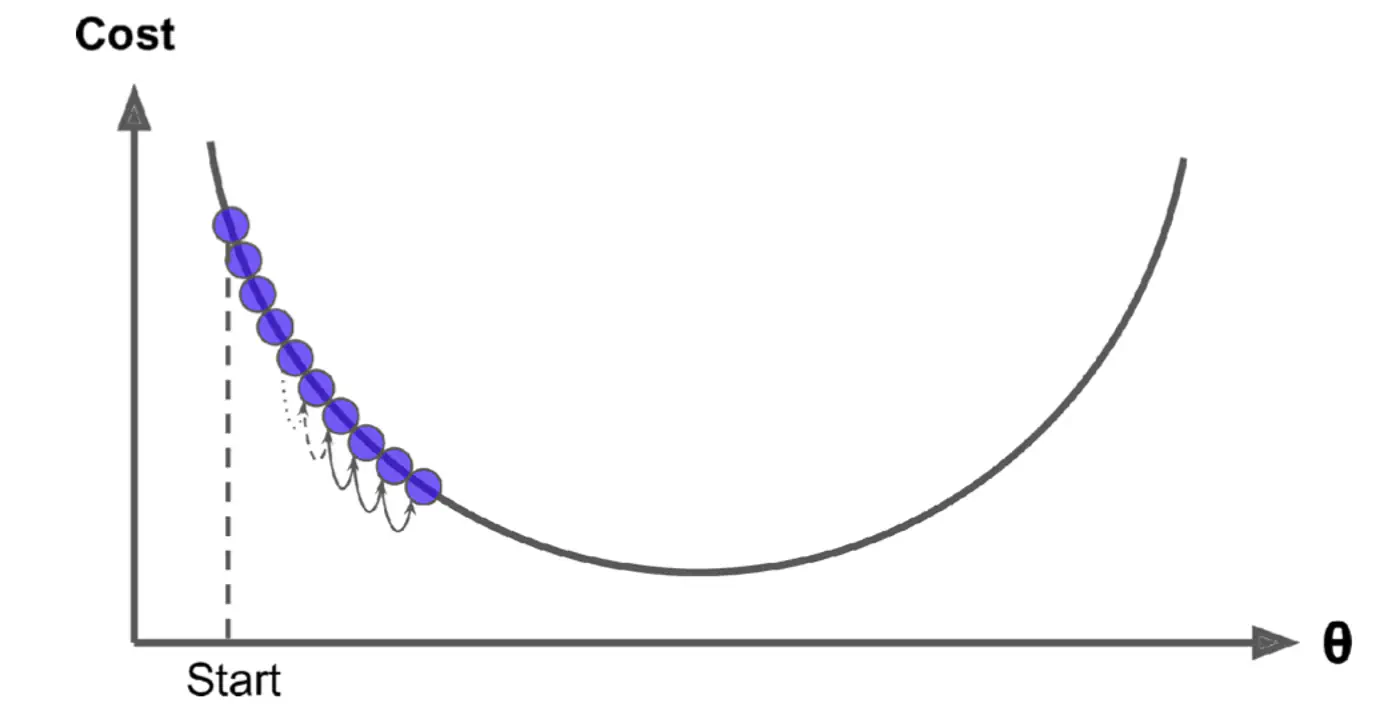
Large \(\eta\) ->
- Learning Rate Schedule:
The learning rate is decayed (reduced) over time.
Large steps initially and fine-tuning near the minimum, e.g., step decay or exponential decay. - Adaptive Learning Rate Methods:
Automatically adjust the learning rate for each parameter ‘w’ based on the history of gradients.
Preferred in modern deep learning as they require less manual tuning, e.g., Adagrad, RMSprop, and Adam.
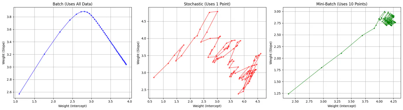
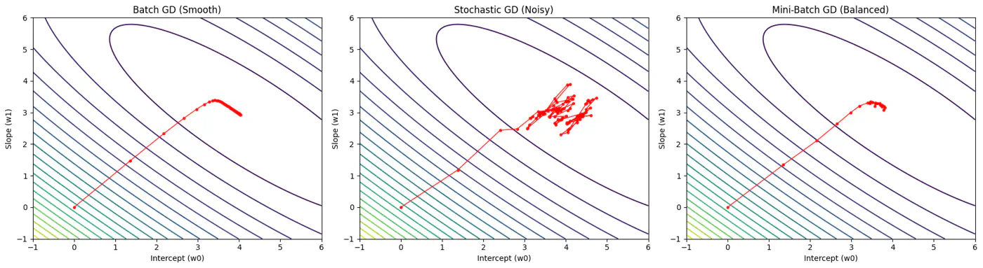
Batch, Stochastic, Mini-Batch are classified by data usage for gradient calculation in each iteration.
- Batch Gradient Descent (BGD): Entire Dataset
- Stochastic Gradient Descent (SGD): Random Point
- Mini-Batch Gradient Descent (MBGD): Subset
Computes the gradient using all the data points in the dataset for parameter update in each iteration.
\[w_{new} = w_{old} - \eta.\text{(average of all ’n’ gradients)}\]🔑Key Points:
- Slow 🐢 steps towards convergence, i.e, TC = O(n).
- Smooth, direct path towards minima.
- Minimum number of steps/iterations.
- Not suitable for large datasets; impractical for Deep Learning, as n = millions/billions.
Uses only 1 data point selected randomly from dataset to compute gradient for parameter update in each iteration.
\[w_{new} = w_{old} - \eta.\text{(gradient at any random data point)}\]🔑Key Points:
- Computationally fastest 🐇 per step; TC = O(1).
- Highly noisy, zig-zag path to minima.
- High variance in gradient estimation makes path to minima volatile, requiring a careful decay of learning rate to ensure convergence to minima.
- Uses small randomly selected subsets of dataset, called mini-batch, (1<k<n), to compute gradient for parameter update in each iteration. \[w_{new} = w_{old} - \eta.\text{(average gradient of ‘k' data points)}\]
🔑Key Points:
- Moderate time ⏰ consumption per step; TC = O(k<n).
- Less noisy, and more reliable convergence than stochastic gradient descent.
- More efficient and faster than batch gradient descent.
- Standard optimization algorithm for Deep Learning.Note: Vectorization on GPUs allows for parallel processing of mini-batches; also GPUs are the reason for the mini-batch size to be a power of 2.
End of Section
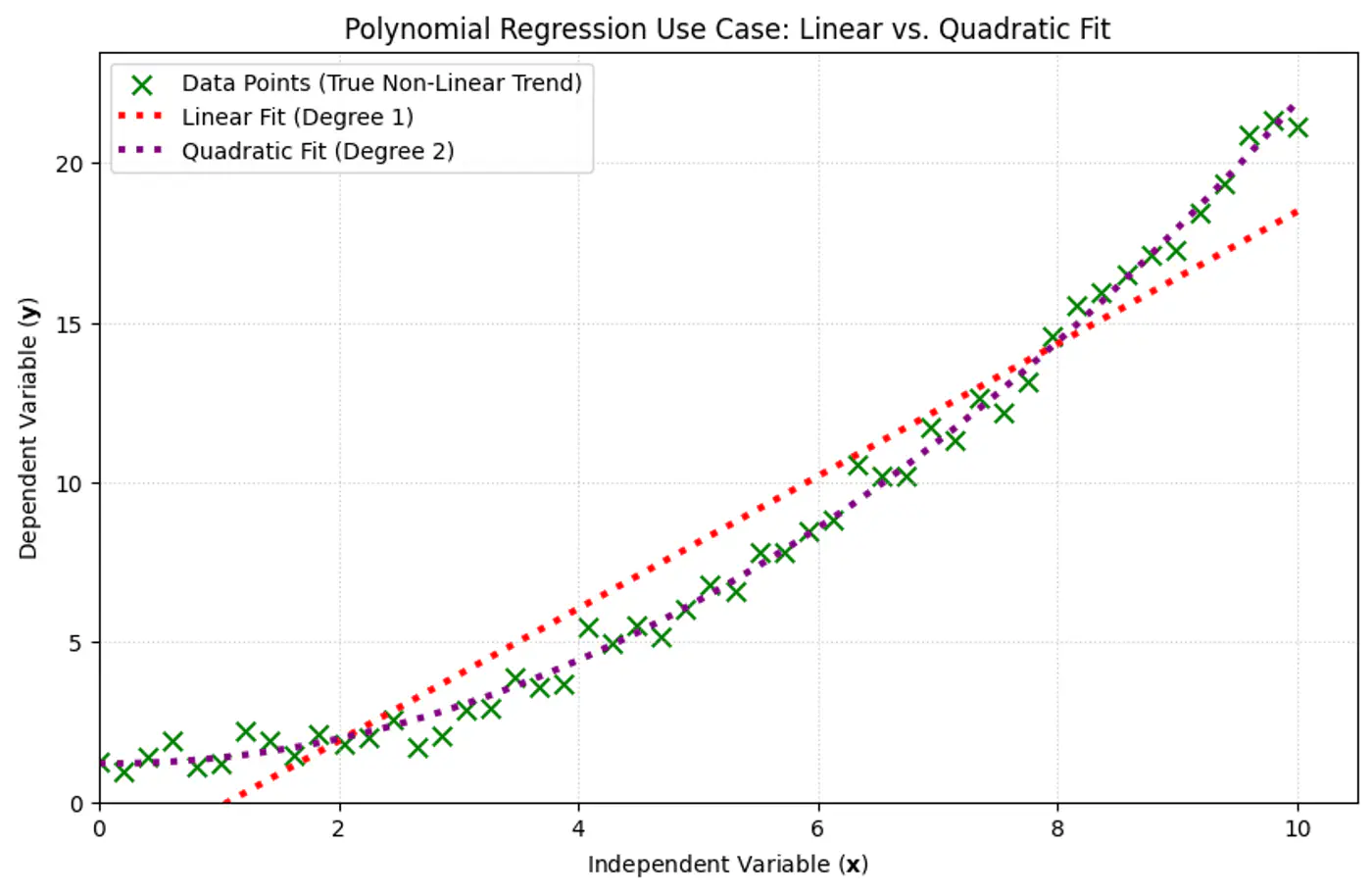
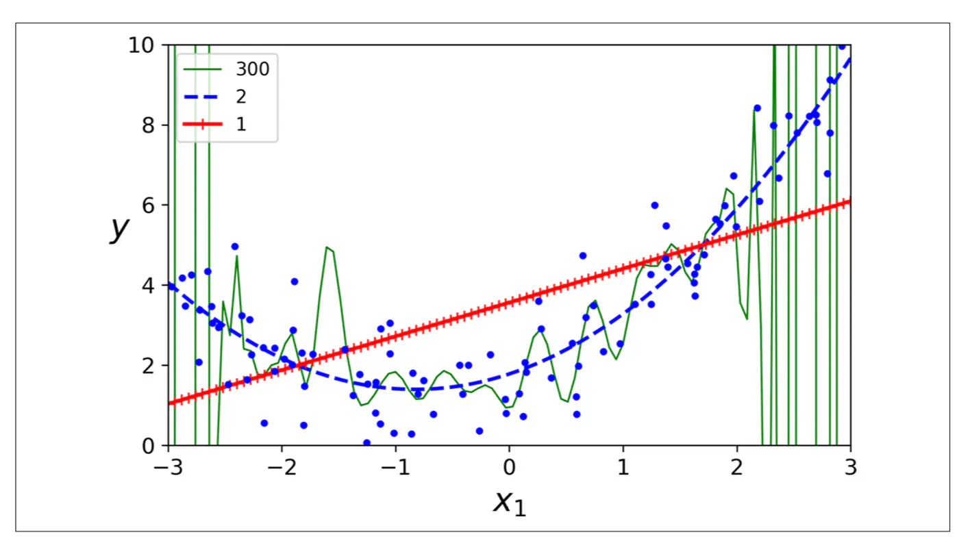
2.1.7 - Polynomial Regression
We can use a linear model to fit non-linear data.
Add powers of each feature as new features, then train a linear model on this extended set of features.
Linear: \(\hat{y_i} = w_0 + w_1x_{i_1} \)
Polynomial (quadratic): \(\hat{y_i} = w_0 + w_1x_{i_1} + w_2x_{i_1}^2\)
Polynomial (n-degree): \(\hat{y_i} = w_0 + w_1x_{i_1} + w_2x_{i_1}^2 +w_3x_{i_1}^3 + \dots + w_nx_{i_1}^n \)
Above polynomial can be re-written as linear equation:
\[\hat{y_i} = w_0 + w_1X_1 + w_2X_2 +w_3X_3 + \dots + w_nX_n \]where, \(X_1 = x_{i_1}, X_2 = x_{i_1}^2, X_3 = x_{i_1}^3, \dots, X_n = x_{i_1}^n\)
=> the model is still linear w.r.t to its parameters/weights \(w_0, w_1, w_2, \dots , w_n \).
e.g:

- Fit a linear model to the data points.
- Plot the errors.
- If the variance of errors is too high, then try polynomial features.
Note: Detect and remove outliers from error distribution.

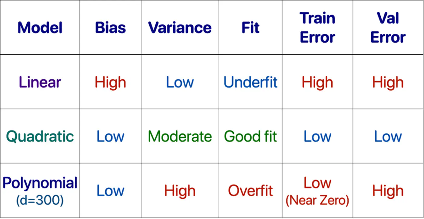
- Polynomial model : Over-fitting ❌
- Linear model : Under-fitting ❌
- Quadratic model: Generalizes best ✅
End of Section
2.1.8 - Data Splitting
- Training Data: Learn model parameters (Textbook + Practice problems)
- Validation Data: Tune hyper-parameters (Mock tests)
- Test Data: Evaluate model performance (Real (final) exam)
Data leakage occurs when information from the validation or test set is inadvertently used to train 🏃♂️ the model.
The model ‘cheats’ by learning to exploit information it should not have access to, resulting in artificially inflated performance metrics during testing 🧪.
- Small datasets(1K-100K): 60/20/20, 70/15/15 or 80/10/10
- Large datasets(>1M): 98/1/1 would suffice, as 1% of 1M is still 10K.
Note: There is no fixed rule, its trial and error.
If there is class imbalance in the dataset, (e.g., 95% class A , 5% class B), a random split might result in the validation set having 99% class A.
Solution: Use stratified sampling to ensure class proportions are maintained across all splits (train️/validation/test).
Note: Non-negotiable for imbalanced data.
- In time-series ⏰ data, divide the data chronologically, not randomly, i.e, training data time ⏰ should precede validation data time ⏰.
- We always train 🏃♂️ on past data to predict future data.
Golden rule: Never look 👀 into the future.
End of Section
2.1.9 - Cross Validation
Do not trust one split of the data; validate across many splits, and average the result to reduce randomness and bias.
Note: Two different splits of the same dataset can give very different validation scores.
Cross-validation is a statistical resampling technique used to evaluate how well a machine learning model generalizes to an independent, unseen dataset.
It works by systematically partitioning the available data into multiple subsets, or ‘folds’, and then training and testing the model on different combinations of these folds.
- K-Fold Cross-Validation
- Leave-One-Out Cross-Validation (LOOCV)
- Shuffle the dataset randomly (except time-series ⏳).
- Split data into k equal subsets(folds).
- Iterate through each unique fold, using it as the validation set.
- Use remaining k-1 fold for training 🏃♂️.
- Take an average of the results.Note: Common choice for k=5 or 10.
- Iteration 1: [V][T][T][T][T]
- Iteration 2: [T][V][T][T][T]
- Iteration 3: [T][T][V][T][T]
- Iteration 4: [T][T][T][V][T]
- Iteration 5: [T][T][T][T][V]
Model is trained 🏃♂️on all data points except one, and then tested 🧪on that remaining single observation.
LOOCV is an extreme case of k-fold cross-validation, where, k=n (number of data points).
Pros:
Useful for small (<1000) datasets.Cons:
Computationally 💻 expensive 💰.
End of Section
2.1.10 - Bias Variance Tradeoff
Mean Squared Error (MSE) = \(\frac{1}{n} \sum_{i=1}^n (y_i - \hat{y_i})^2\)
Total Error = Bias^2 + Variance + Irreducible Error
- Bias = Systematic Error
- Bias measures how far the average prediction of a model is from the true value.
- Variance = Sensitivity to Data
- Variance measures how much the predictions of a model vary for different training datasets.
- Irreducible Error = Sensor noise, Human randomness
- Inherent uncertainty in the data generation process itself and cannot be reduced by any model.
Systematic error from overly simplistic assumptions or strong opinion in the model.
e.g. House 🏠 prices 💰 = Rs. 10,000 * Area (sq. ft).
Note: This is over simplified view, because it ignores, amenities, location, age, etc.
Error from sensitivity to small fluctuations 📈 in the data.
e.g. Deep neural 🧠 network trained on a small dataset.
Note: Memorizes everything, including noise.
Say a house 🏠 in XYZ street was sold for very low price 💰.
Reason: Distress selling (outlier), or incorrect entry (noise).
Note: Model will make wrong(lower) price 💰predictions for all houses in XYZ street.
Goal 🎯 is to minimize total error.
Find a sweet-spot balance ⚖️ between Bias and Variance.
A good model ‘generalizes’ well, i.e.,
- Is not too simple or has a strong opinion.
- Does not memorize 🧠 everything in the data, including noise.
- Make model more complex.
- Add more features, add polynomial features.
- Decrease Regularization.
- Train 🏃♂️longer, the model has not yet converged.
- Add more data (most effective).
- Harder to memorize 🧠 1 million examples than 100.
- Use data augmentation, if getting more data is difficult.
- Increase Regularization.
- Early stopping 🛑, prevents memorization 🧠.
- Dropout (DL), randomly kill neurons, prevents co-adaptation.
- Use Ensembles.
- Averaging reduces variance.
Note: Co-adaptation refers to a phenomenon where neurons in a neural network become highly dependent on each other to detect features, rather than learning independently.
End of Section
2.1.11 - Regularization
Over-Fitting happens when we have a complex model that creates highly erratic curve to fit every single data point, including the random noise.
- Excellent performance on training 🏃♂️ data, but poor performance on unseen data.
- Penalty for overly complex models, i.e, models with excessively large or numerous parameters.
- Focus on learning general patterns rather than memorizing 🧠 everything, including noise in training 🏃♂️data.
Set of techniques that prevents over-fitting by adding a penalty term to the model’s loss function.
\[ J_{reg}(w) = J(w) + \lambda.\text{Penalty(w)} \]\(\lambda\) = Regularization strength hyper parameter, bias-variance tradeoff knob.
- High \(\lambda\): High ⬆️ penalty, forces weights towards 0, simpler model.
- Low \(\lambda\): Weak ⬇️ penalty, closer to un-regularized model.
- By intentionally simplifying a model (shrinking weights) to reduce its complexity, which prevents it from overfitting.
- Penalty pulls feature weights closer to zero, making the model less faithful representation of the training data’s true complexity.
- L2 Regularization (Ridge Regression)
- L1 Regularization (Lasso Regression)
- Elastic Net Regularization
- Early Stopping
- Dropout (Neural Networks)
- Penalty term: \(\ell_2\) norm - penalizes large weights quadratically.
- Pushes the weights close to 0 (not exactly 0), making models more stable by distributing importance across weights.
- Splits feature importance across co-related features.
- Use case: Best when most features are relevant and co-related.
- Also known as Ridge regression or Tikhonov regularization.
- Penalty term: \(\ell_1\) norm.
- Shrinks some weights exactly to 0, effectively performing feature selection, giving sparse solutions.
- For a group of highly co-related features, arbitrarily selects one feature and shrinks others to 0.
- Use case: Best when using high-dimensional datasets (d»n) where we suspect many features are irrelevant or redundant, or when model interpretability matters.
- Also known as Lasso (Least Absolute Shrinkage and Selection Operator) regression.
- Computational hack: \(\frac{\partial{|w_j|}}{\partial{w_j}} = 0\), since absolute function is not differentiable at 0.
- Penalty term : linear combination of and norm.
- Sparsity(feature-selection) of L1 and stability/grouping effect of L2 regularization.
- Use case: Best when we have high dimensional data with correlated features and we want sparse and stable solution.
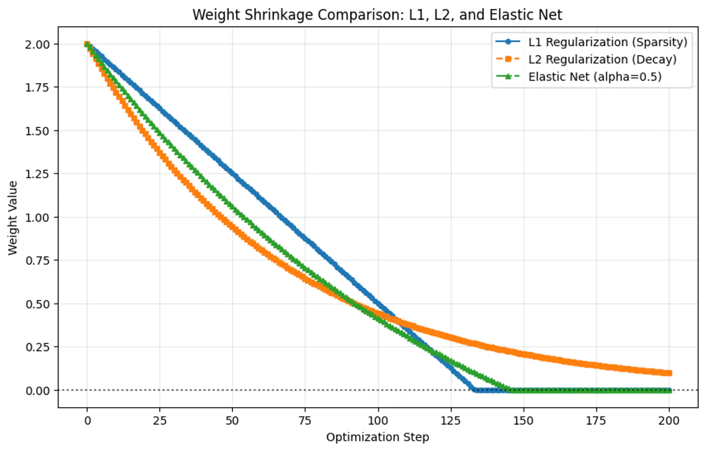
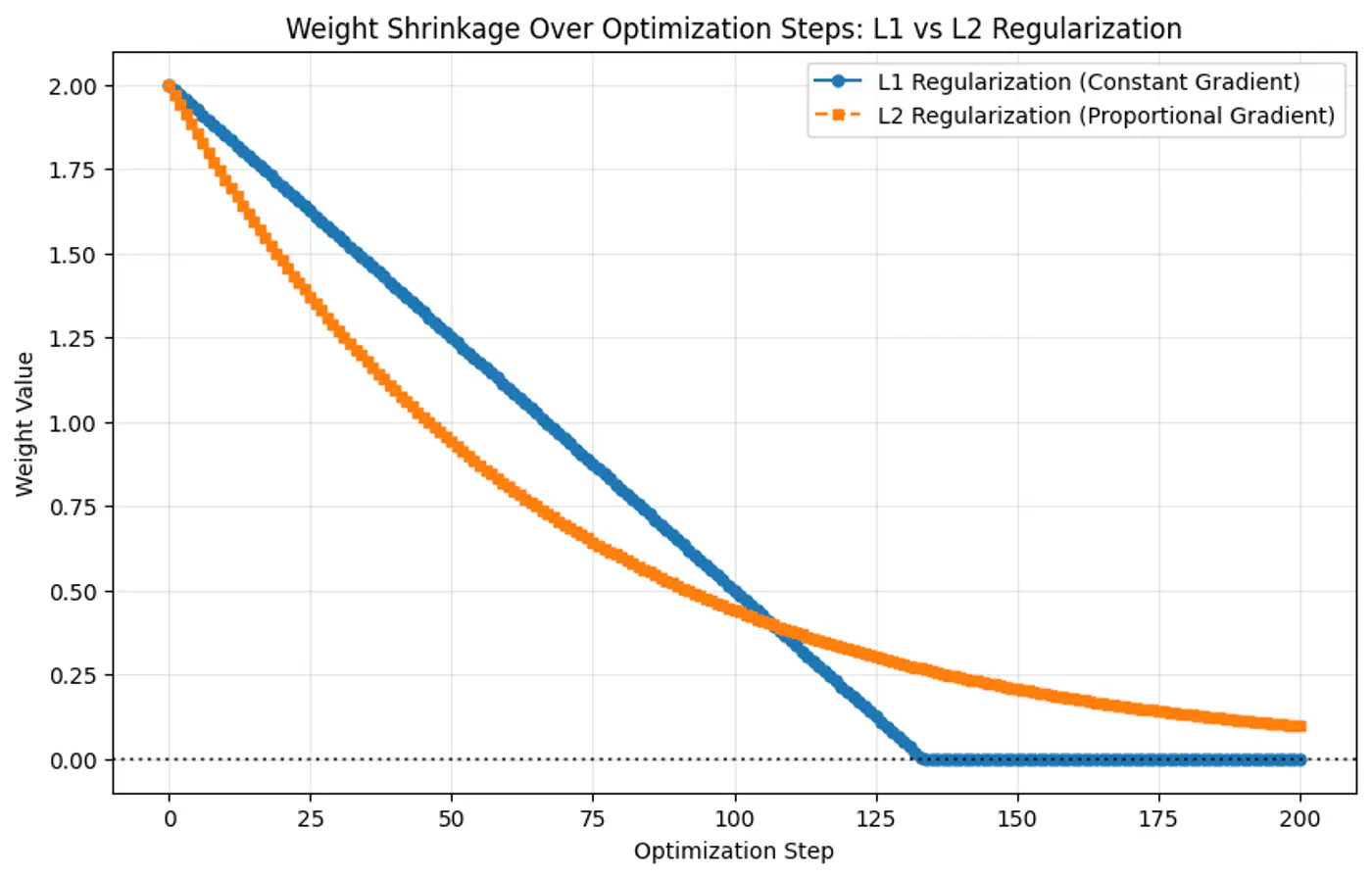
- Because the gradient of L1 penalty (absolute function) is a constant value, i.e, \(\pm 1\), this means a constant reduction in weight at each step, making it gradually reach to 0 in finite steps.
- Whereas, the derivative of L2 penalty is proportional to the weight (\(2w_j\)) and as the weight reaches close to 0, the gradient also becomes very small, this means that the weight will become very close to 0, but not exactly equal to 0.
End of Section
2.1.12 - Regression Metrics
MAE = \(\frac{1}{n} \sum_{i=1}^n |y_i - \hat{y_i}|\)
- Treats each error equally.
- Robust to outliers.
- Not differentiable x=0.
- Using gradient descent requires computational hack.
- Easy to interpret, as same units as target variable.
MSE = \(\frac{1}{n} \sum_{i=1}^n (y_i - \hat{y_i})^2\)
- Heavily penalizes large errors.
- Sensitive to outliers.
- Differentiable everywhere.
- Used by gradient descent and most other optimization algorithms.
- Difficult to interpret, as it has squared units.
RMSE = \(\sqrt{\frac{1}{n} \sum_{i=1}^n (y_i - \hat{y_i})^2}\)
- Easy to interpret, as it has same units as target variable.
- Useful when we need outlier-sensitivity of MSE but the interpretability of MAE.
Measures improvement over mean model.
\[ R^2 = 1 - \frac{SS_{res}}{SS_{tot}} = 1 - \frac{\sum_{i=1}^n (y_i - \hat{y_i})^2}{\sum_{i=1}^n (y_i - \bar{y_i})^2} \]Good R^2 value depends upon the use case, e.g. :
- Car 🚗 sale, R =0.8 is good enough.
- Cancer 🧪 prediction R 0.95, as life depends on it.
Range of values:
- Best value = 1
- Baseline value = 0
- Worst value = \(- \infty\)
Note: Example for bad model is all the points lie along x-axis and model predicts y-axis.
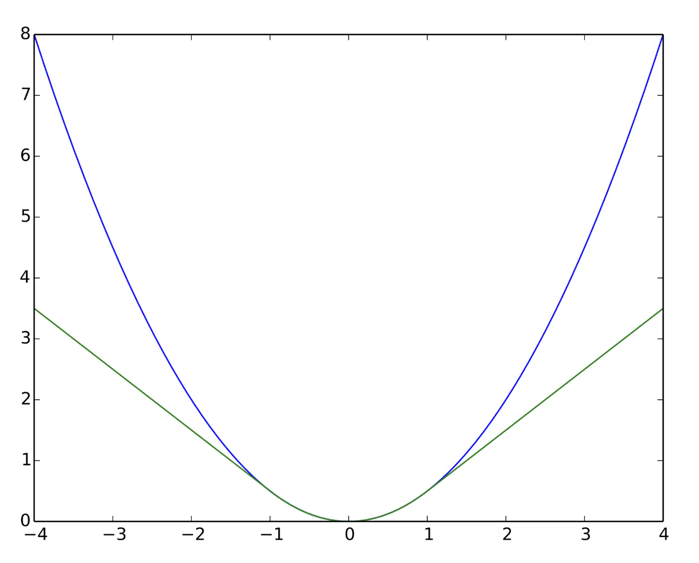
Quadratic for small errors; Linear for large errors.
\[ L_{\delta}(y, \hat{y}) = \begin{cases} \frac{1}{2}(y - \hat{y})^2 & \text{for } |y - \hat{y}| \le \delta \\ \\ \delta (|y - \hat{y}| - \frac{1}{2}\delta) & \text{otherwise} \end{cases} \]- Robust to outliers.
- Differentiable at 0; smooth convergence to minima.
- Delta (\(\delta\)) knob(hyper parameter) to control.
- \(\delta\) high: MSE
- \(\delta\) low: MAE
Note: Tune \(\delta\): MAE, for outliers > \(\delta\); MSE, for small errors < \(\delta\).
e.g: = 95th percentile of errors or 1.35\(\sigma\) for standard Gaussian data.
Huber loss (Green) and Squared loss (blue)
End of Section
2.1.13 - Assumptions
Linear Regression works reliably only when certain key 🔑 assumptions about the data are met.
- Linearity
- Independence of Errors (No Auto-Correlation)
- Homoscedasticity (Equal Variance)
- Normality of Errors
- No Multicollinearity
- No Endogeneity (Target not correlated with the error term)
Relationship between features and target 🎯 is linear in parameters.
Note: Polynomial regression is linear regression.
\(y=w_0 +w_1x_1+w_2x_2^2 + w_3x_3^3\)
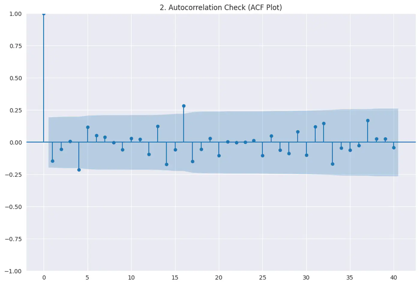
Residuals (errors) should not have a visible pattern or correlation with one another (most common in time-series ⏰ data).
Risk:
If errors are correlated, standard errors will be underestimated, making variables look ‘statistically significant’ when they are not.
Test:
Durbin–Watson test
Autocorrelation plots (ACF)
Residuals vs time
Constant variance of errors; Var(ϵ|X)=σ
Risk:
Standard errors become biased, leading to unreliable hypothesis tests (t-tests, F-tests).
Test:
- Breusch–Pagan test
- White test
Fix:
- Log transform
- Weighted Least Squares(WLS)
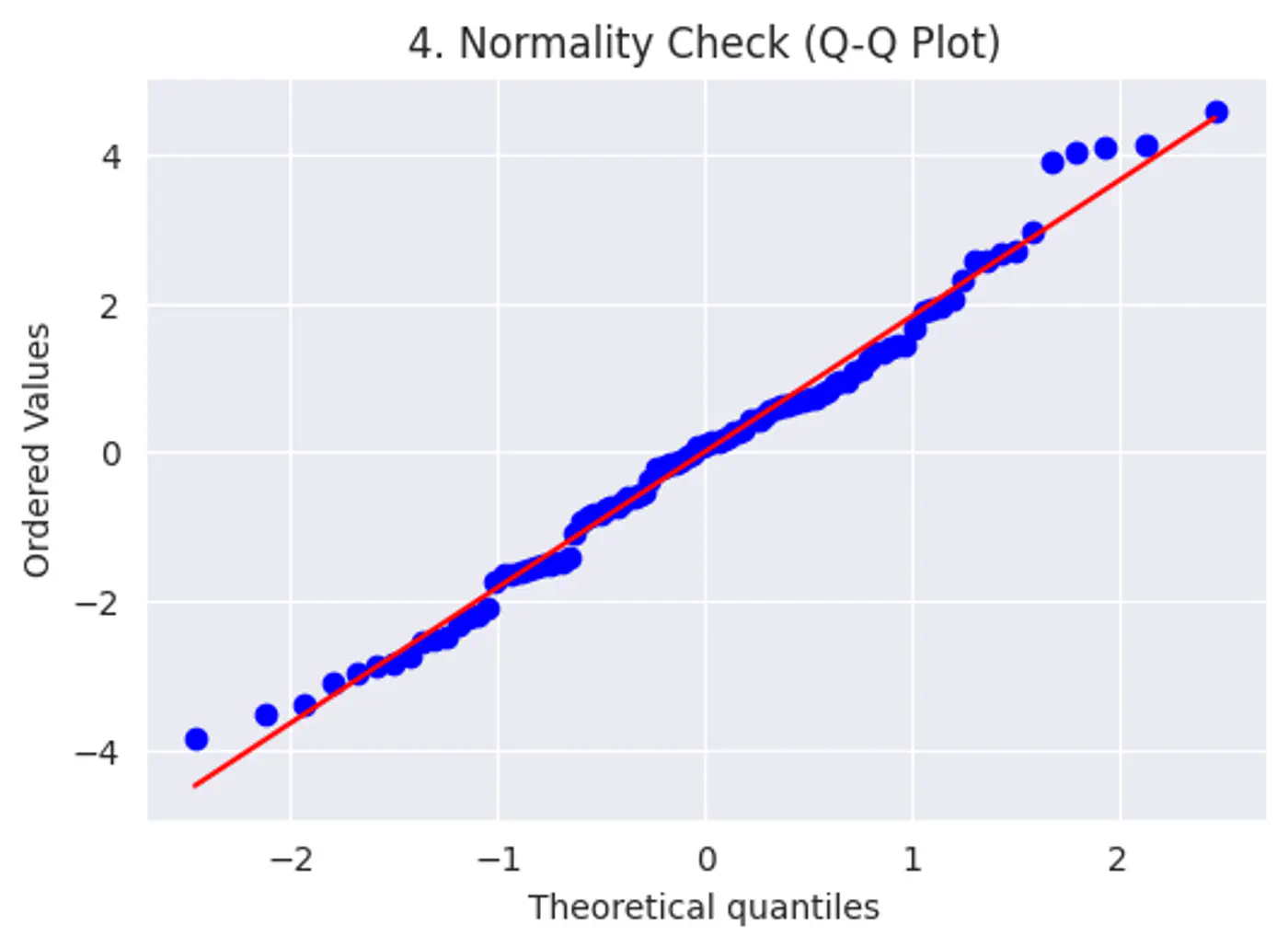
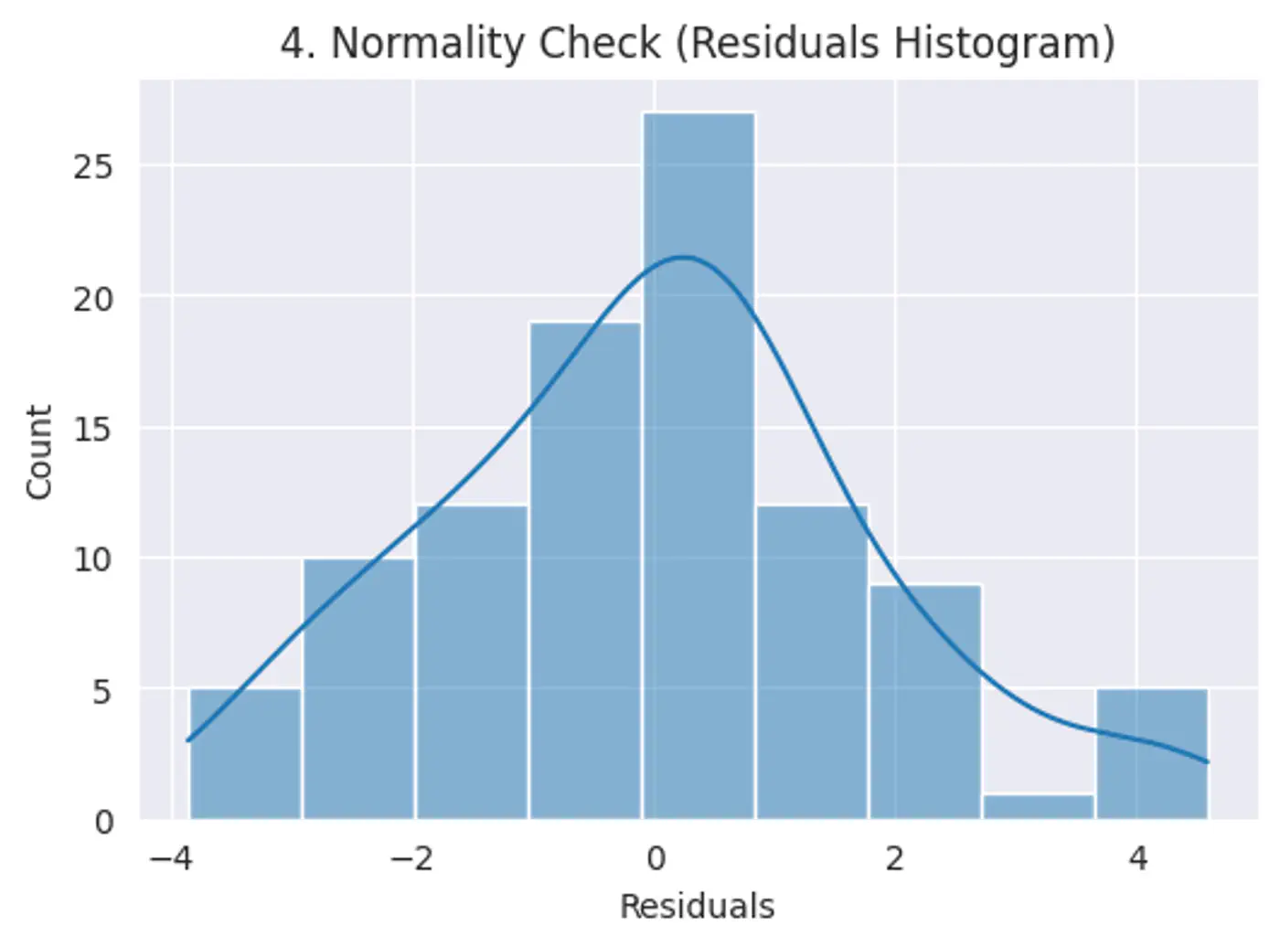
Error terms should follow a normal distribution; (Required for small datasets.)
Note: Because of Central Limit Theorem, with a large enough sample size, this becomes less critical for estimation.
Risk: Hypothesis testing (calculating p-values and confidence intervals), we assume the error terms follow a normal distribution.
Test:
Q-Q plot
Shapiro-Wilk Test
Features should not be highly correlated with each other.
Risk:
- High correlation makes it difficult to determine the unique, individual impact of each feature. This leads to high variance in model parameter estimates, small changes in data cause large swings in parameters.
- Model interpretability issues.
Test:
- Variance Inflation Factor(VIF)VIF > 5 → concern, VIF > 10 → serious issue
Fix:
- PCA
- Remove redundant features
Error term must be uncorrelated with the features; E[ϵ|X] = 0
Risk:
- Parameters will be biased and inconsistent.
Test:
- Hausman Test
- Durbin-Wu-Hausman (DWH) Test
Fix:
- Controlled experiments.
End of Section
2.2.1 - Binary Classification
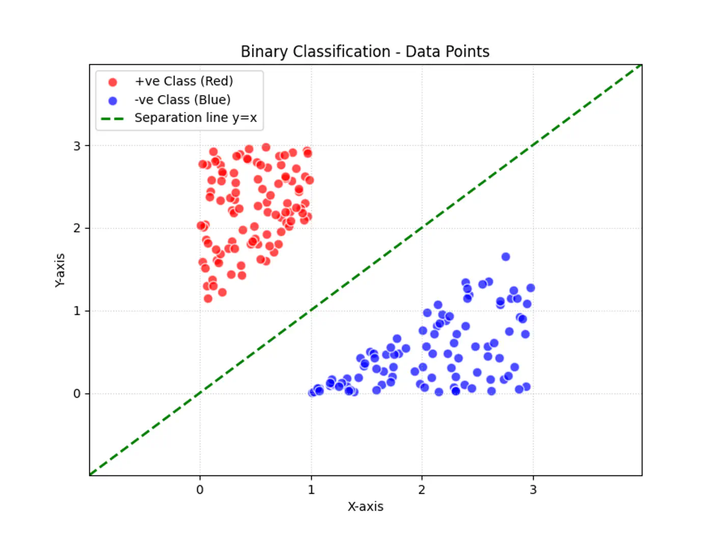
Linear regression tries to find the best fit line, but we want to find the line or decision boundary that clearly separates the two classes.
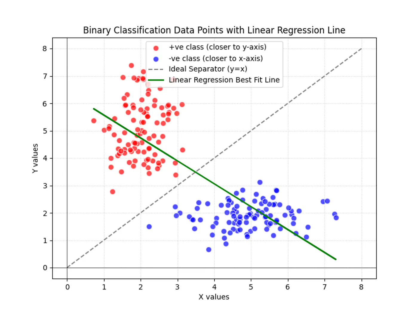
Find the decision boundary, i.e, the equation of the separating hyperplane.
\[z=w^{T}x+w_{0}\]Value of \(z = \mathbf{w^Tx} + w_0\) tells us how far is the point from the decision boundary and on which side.
Note: Weight 🏋️♀️ vector ‘w’ is normal/perpendicular to the hyperplane, pointing towards the positive class (y=1).
- For points exactly on the decision boundary \[z = \mathbf{w^Tx} + w_0 = 0 \]
- Positive (+ve) labeled points \[ z = \mathbf{w^Tx} + w_0 > 0 \]
- Negative (-ve) labeled points \[ z = \mathbf{w^Tx} + w_0 < 0 \]
So we need a link 🔗 to transform the geometric distance to probability.
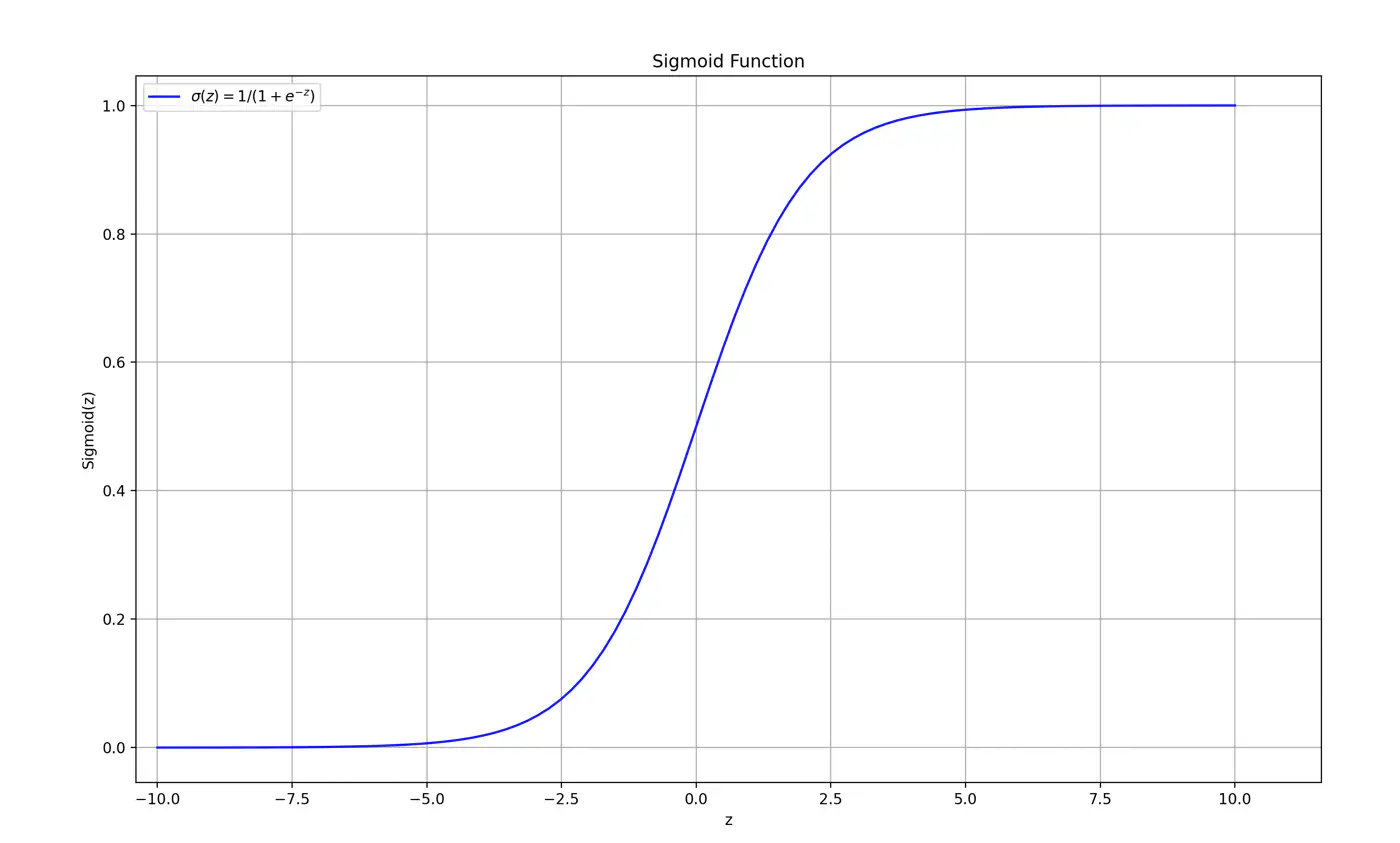
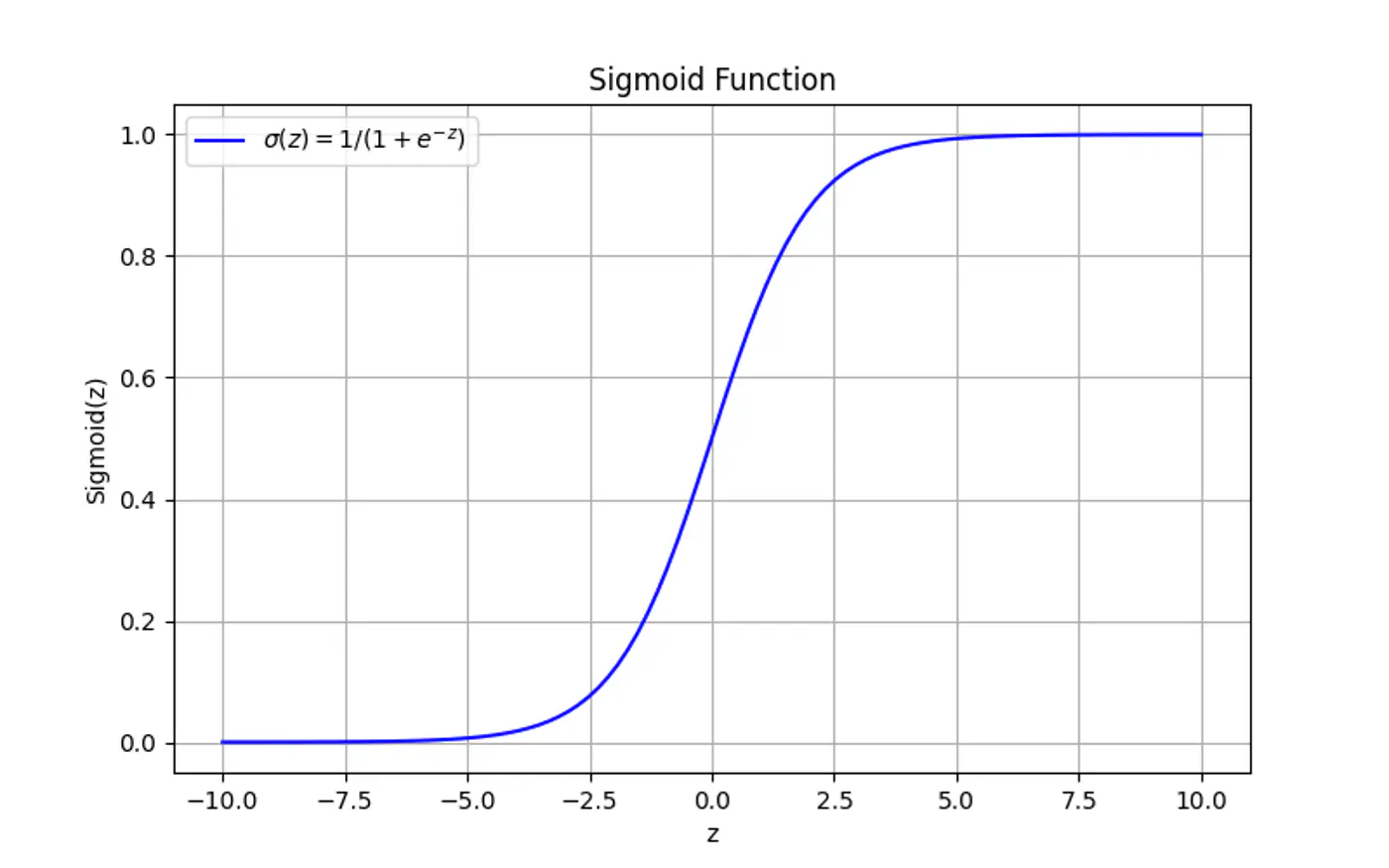
Maps the output of a linear equation to a value between 0 and 1, allowing the result to be interpreted as a probability.
\[\hat{y} = \sigma(z) = \frac{1}{1 + e^{-z}}\]If the distance ‘z’ is large and positive, \(\hat{y} \approx 1\) (High confidence).
If the distance ‘z’ is 0, \(\hat{y} = 0.5\) (Maximum uncertainty).
End of Section
2.2.2 - Log Loss
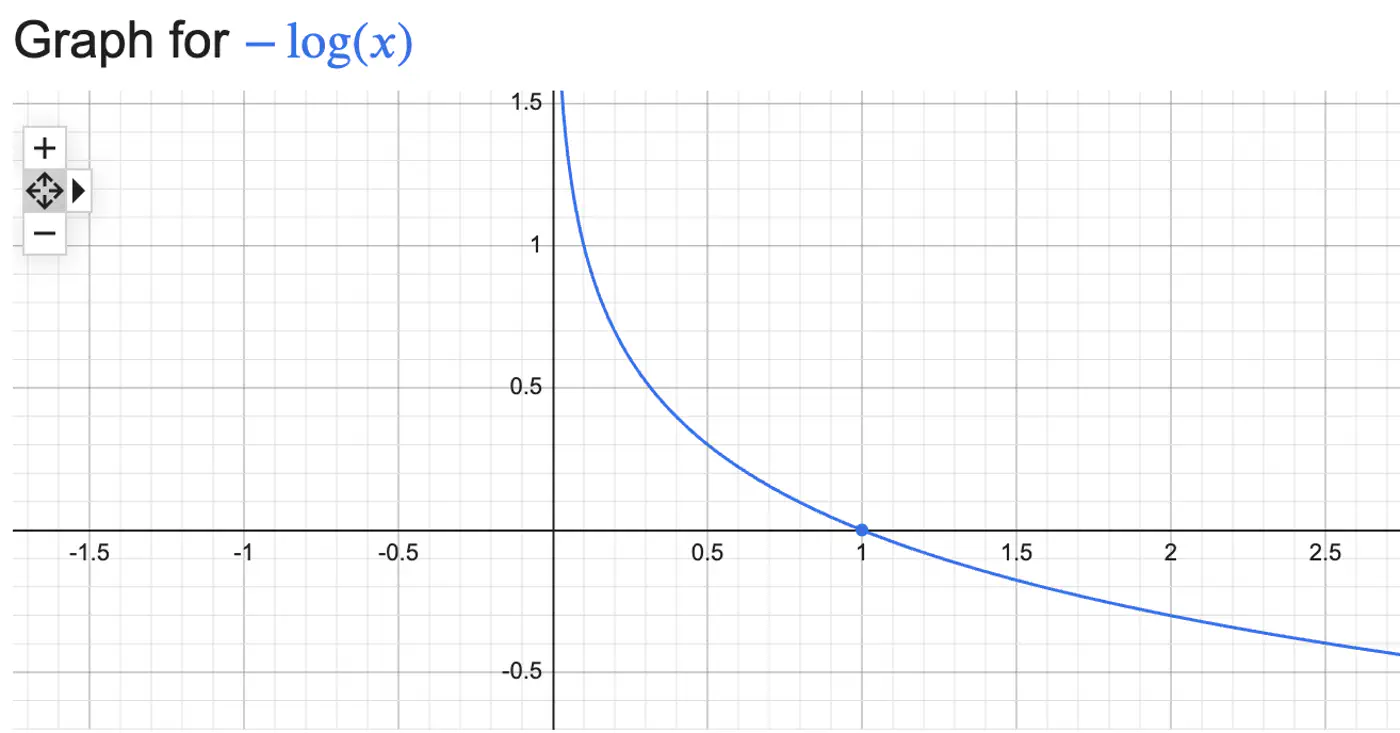
Log Loss = \(\begin{cases} -log(\hat{y_i}) & \text{if } y_i = 1 \\ \\ -log(1-\hat{y_i}) & \text{if } y_i = 0 \end{cases} \)
Combining the above 2 conditions into 1 equation gives:
Log Loss = \(-[y_ilog(\hat{y_i}) + (1-y_i)log(1-\hat{y_i})]\)
We need to find the weights 🏋️♀️ ‘w’ that minimize the cost 💵 function.
- Weight update: \[w_{new}=w_{old}-η.\frac{∂J(w)}{∂w_{old}}\]
We need to find the gradient of log loss w.r.t weight ‘w’.
Chain Rule:
\[\frac{\partial{J(w)}}{\partial{w}} = \frac{\partial{J(w)}}{\partial{\hat{y}}}.\frac{\partial{\hat{y}}}{\partial{z}}.\frac{\partial{z}}{\partial{w}}\]- Cost Function: \(J(w) = -\frac{1}{n}\sum [y_ilog(\hat{y_i}) + (1-y_i)log(1-\hat{y_i})]\)
- Prediction: \(\hat{y} = \sigma(z) = \frac{1}{1 + e^{-z}}\)
- Distance of Point: \(z = \mathbf{w^Tx} + w_0\)
How loss changes w.r.t prediction ?
\[ \begin{align*} \frac{\partial{J(w)}}{\partial{\hat{y}}} &= - [\frac{y}{\hat{y}} - \frac{1-y}{1-\hat{y}}] \\ &= -[\frac{y- \cancel{y\hat{y}} -\hat{y} + \cancel{y\hat{y}}}{\hat{y}(1-\hat{y})}] \\ \therefore \frac{\partial{J(w)}}{\partial{\hat{y}}} &= \frac{\hat{y} - y}{\hat{y}(1-\hat{y})} \end{align*} \]How prediction changes w.r.t distance ?
\[ \begin{align*} \frac{\partial{\hat{y}}}{\partial{z}} &= \frac{\partial{\sigma(z)}}{\partial{z}} = \sigma'(z) \\ \sigma'(z) &= \sigma(z)(1-\sigma(z)) \\ \therefore \frac{\partial{\hat{y}}}{\partial{z}} &= \hat{y}(1-\hat{y}) \end{align*} \]from equations (1) & (2):
\[ \begin{align*} \because \frac{\partial{\sigma(z)}}{\partial{z}} &= \frac{\partial{\sigma(z)}}{\partial{u}}. \frac{\partial{u}}{\partial{z}} \\ \implies \frac{\partial{\sigma(z)}}{\partial{z}} &= - \frac{1}{(1 + e^{-z})^2}. -e^{-z} = \frac{e^{-z}}{(1 + e^{-z})^2} \\ 1 - \sigma(z) & = 1 - \frac{1}{1 + e^{-z}} = \frac{e^{-z}}{1 + e^{-z}} \\ \frac{\partial{\sigma(z)}}{\partial{z}} &= \frac{1}{1 + e^{-z}}.\frac{e^{-z}}{1 + e^{-z}} \\ \therefore \frac{\partial{\sigma(z)}}{\partial{z}} &= \sigma(z).(1-\sigma(z)) \end{align*} \]How distance changes w.r.t weight 🏋️♀️ ?
\[ \frac{\partial{z}}{\partial{w}} = \mathbf{x} \]\[\because \frac{\partial{(a^T\mathbf{x})}}{\partial{\mathbf{x}}} = a\]Chain Rule:
\[ \begin{align*} \frac{\partial{J(w)}}{\partial{w}} &= \frac{\partial{J(w)}}{\partial{\hat{y}}}.\frac{\partial{\hat{y}}}{\partial{z}}.\frac{\partial{z}}{\partial{w}} \\ &= \frac{\hat{y} - y}{\cancel{\hat{y}(1-\hat{y})}}.\cancel{\hat{y}(1-\hat{y})}.x \\ \therefore \frac{\partial{J(w)}}{\partial{w}} &= (\hat{y} - y).x \end{align*} \]Gradient = Error x Input
- Error = \((\hat{y_i}-y_i)\): how far is prediction from the truth?
- Input = \(x_i\): contribution of specific feature to the error.
Weight update:
\[w_{new} = w_{old} - \eta. \sum_{i=1}^n (\hat{y_i} - y_i).x_i\]Mean Squared Error (MSE) can not be used to quantify error/loss in binary classification because:
- Convexity : MSE combined with Sigmoid is non-convex, so, Gradient Descent can get trapped in local minima.
- Penalty: MSE does not appropriately penalize mis-classifications in binary classification.
- e.g: If actual value is class 1 but the model predicts class 0, then MSE = \((1-0)^2 = 1\), which is very low, whereas log loss = \(-log(0) = \infty\)
End of Section
2.2.3 - Regularization
The weights 🏋️♀️ will tend towards infinity, preventing a stable solution.
The model tries to make probabilities exactly 0 or 1, but the sigmoid function never reaches these limits, leading to extreme weights 🏋️♀️ to push probabilities near the extremes.
Distance of Point: \(z = \mathbf{w^Tx} + w_0\)
Prediction: \(\hat{y} = \sigma(z) = \frac{1}{1 + e^{-z}}\)
Log loss: \(-[y_ilog(\hat{y_i}) + (1-y_i)log(1-\hat{y_i})] \)
Model becomes perfectly accurate on training 🏃♂️data but fails to generalize, performing poorly on unseen data.
Adds a penalty term to the loss function, discouraging weights 🏋️♀️ from becoming too large.
End of Section
2.2.4 - Log Odds
Odds compare the likelihood of an event happening vs. not happening.
Odds = \(\frac{p}{1-p}\)
- p = probability of success
In logistic regression we assume that Log-Odds (the log of the ratio of positive class to negative class) is a linear function of inputs.
Log-Odds (Logit) = \(log_e \frac{p}{1-p}\)
Log Odds = \(log_e \frac{p}{1-p} = z\)
\[z=w^{T}x+w_{0}\]\[ \begin{align*} &log_{e}(\frac{p}{1-p}) = z \\ &⟹\frac{p}{1-p} = e^{z} \\ &\implies p = e^z - p.e^z \\ &\implies p = \frac{e^z}{1+e^z} \\ &\text { divide numerator and denominator by } e^z \\ &\implies p = \frac{1}{1+e^{-z}} \quad \text { i.e, Sigmoid function} \end{align*} \]- Probability: 0 to 1
- Odds: 0 to + \(\infty\)
- Log Odds: -\(\infty\) to +\(\infty\)
End of Section
2.2.5 - Probabilistic Interpretation
We assume that our target variable ‘y’ follows a Bernoulli distribution, i.e, has exactly 2 outputs success/failure.
- P(Y=1|X) = p
- P(Y=0|X) = 1- p
Combining above 2 into 1 equation gives:
- P(Y=y|X) = \(p^y(1-p)^{1-y}\)
‘Find the most plausible explanation for what I see.’
We want to find the weights 🏋️♀️‘w’ that maximize the likelihood of seeing the data.
- Data, D = \(\{ (x_i, y_i)_{i=1}^n , \quad y_i \in \{0,1\} \}\)
We do this by maximizing likelihood function.
Assumption: Training data is I.I.D.
A common simplification is to maximize the log-likelihood function instead, which converts the product into a sum.
Note: Log is a strictly monotonically increasing function.
Maximizing the log-likelihood is same as minimizing the negative of log-likelihood.
\[ \begin{align*} \underset{w}{\mathrm{max}}\ log\mathcal{L}(w) &= \underset{w}{\mathrm{min}} - log\mathcal{L}(w) \\ \underset{w}{\mathrm{min}} - log\mathcal{L}(w) &= - \sum_{i=1}^n [ y_ilog(p_i) + (1-y_i)log(1-p_i)] \\ \underset{w}{\mathrm{min}} - log\mathcal{L}(w) &= \text {Log Loss} \end{align*} \]End of Section
2.3.1 - KNN Introduction
- Parametric models:
- Rely on assumption that relationships between data points are linear.
- For polynomial regression we need to find the degree of polynomial.
- Training:
- We need to train 🏃♂️the model for prediction.
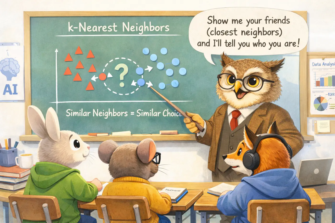
Simple: Intuitive way to classify data or predict values by finding similar existing data points (neighbors).
Non-Parametric: Makes no assumptions about the underlying data distribution.
No Training Required: KNN is a ‘lazy learner’, it does not require a formal training 🏃♂️ phase.

Given a query point \(x_q\) and a dataset, D = {\((x_i,y_i)_{i=1}^n, \quad x_i,y_i \in \mathbb{R}^d\)}, the algorithm finds a set of ‘k’ nearest neighbors \(\mathcal{N}_k(x_q) \subseteq D\).
Inference:
- Choose a value of ‘k’ (hyper-parameter); odd number.
- Calculate distance (Euclidean, Cosine etc.) between and every point in dataset and store in a distance list.
- Sort the distance list in ascending order; choose top ‘k’ data points.
- Make prediction:
- Classification: Take majority vote of ‘k’ nearest neighbors and assign label.
- Regression: Take the mean/median of ‘k’ nearest neighbors.
Note: Store entire dataset.
- Storing Data: Space Complexity: O(nd)
- Inference: Time Complexity ⏰: O(nd + nlogn)
Explanation:
- Distance to all ’n’ points in ‘d’ dimensions: O(nd)
- Sorting all ’n’ data points : O(nlogn)
Note: Brute force 🔨 KNN is unacceptable when ’n’ is very large, say billions.
End of Section
2.3.2 - KNN Optimizations
Naive KNN needs some improvements to fix some of its drawbacks.
- Standardization
- Distance-Weighted KNN
- Mahalanobis Distance
⭐️Say one feature is ‘Annual Income’ (0-1M), and another feature is ‘Years of Experience’ (0-40).
👉The Euclidean distance will be almost entirely dominated by income 💵.
💡So, we do standardization of each feature, such that it has a mean, \(\mu\)=0 and variance,\(\sigma\)=1.
\[z=\frac{x-\mu}{\sigma}\]⭐️Vanilla KNN treats the 1st nearest neighbor and the k-th nearest neighbor as equal.
💡A neighbor that is 0.1units away should have more influence than a neighbor that is 10 units away.
👉We assign weight 🏋️♀️ to each neighbor; most common strategy is inverse of squared distance.
\[w_i = \frac{1}{d(x_q, x_i)^2 + \epsilon}\]Improvements:
- Noise/Outlier: Reduces the impact of ‘noise’ or ‘outlier’ (distant neighbors).
- Imbalanced Data: Closer points dominate, mitigating impact of imbalanced data.
- e.g: If you have a query point surrounded by 2 very close ‘Class A’ points and 3 distant ‘Class B’ points, weighted 🏋️♀️ KNN will correctly pick ‘Class A'.
⭐️Euclidean distance makes assumption that all the features are independent and provide unique information.
💡‘Height’ and ‘Weight’ are highly correlated.
👉If we use Euclidean distance, we are effectively ‘double-counting’ the size of the person.
🏇Mahalanobis distance measures distance in terms of standard deviations from the mean, accounting for the covariance between features.
\[d(x, y) = \sqrt{(x - y)^T \Sigma^{-1} (x - y)}\]\(\Sigma\): Covariance matrix of the data
- If \(\Sigma\) is identity matrix, Mahalanobis distance reduces to Euclidean distance.
- If \(\Sigma\) is a diagonal matrix, Mahalanobis distance reduces to Normalized Euclidean distance.
🦀Naive KNN shifts all computation 💻 to inference time ⏰, and it is very slow.
- To find the neighbor for one query, we must touch every single bit of the ‘nxd’ matrix.
- If n=10^9,a single query would take seconds, but we need milliseconds.
- Distance Weighted KNN
- K-D Trees (d<20): Recursively partitions space into axis-aligned hyper-rectangles. O(log N ) search.
- Ball Trees : High dimensional data; Haversine distance for geospatial 🌎 data.
- Approximate Nearest Neighbors (ANN)
- Locality Sensitive Hashing (LSH): Uses ‘bucketizing’ 🗑️ hashes. Points that are close have a high probability of having the same hash.
- Hierarchical Navigable Small World (HNSW); Graph of vectors; Search is a ‘greedy walk’ across levels.
- Product Quantization (Reduce memory 🧠 footprint 👣 of high dimensional vectors)
- ScaNN (Google)
- FAISS (Meta)
- Dimensionality Reduction (Mitigate ‘Curse of Dimensionality’)
- PCA
End of Section
2.3.3 - Curse Of Dimensionality
While Euclidean distance(L norm) is the most frequently discussed, ‘Curse of Dimensionality’ impacts all Minkowski norms (\(L_p\))
\[L_p = (\sum |x_i|^p)^{\frac{1}{p}} \]Note: ‘Curse of Dimensionality’ is largely a function of the exponent (p) in the distance calculation.
Coined 🪙 by mathematician John Bellman in the 1960s while studying dynamic programming.
High dimensional data created following challenges:
- Distance Concentration
- Data Sparsity
- Exponential Sample Requirement
💡Consider a hypercube in d-dimensions of side length = 1; Volume = \(1^d\) = 1
🧊 A smaller inner cube with side length = 1 - \(\epsilon\) ; Volume = \((1 -\epsilon)^d\)
🧐 This implies that almost all the volume of the high-dimensional cube lies near the ‘crust’.
👉e.g: if \(\epsilon\)= 0.01, d = 500; Volume of inner cube = \((1 -0.01)^{500}\) = \(0.99^{500}\) = 0.006 = 0.6%
🤔Consequently, all points become nearly equidistant, and the concept of ‘nearest’ or ‘neighborhood’ loses
its meaning.
⭐️The volume of the feature space increases exponentially with each added dimension.
👉To maintain the same data density found in a 1D space with 10 points, we would need \(10^{10}\)(10 billion) points in 10D space.
💡Because real-world datasets are rarely this large, the data becomes “sparse,” making it difficult to find truly similar neighbors.
⭐️To maintain a reliable result, the amount of training data needed must grow exponentially with the number of dimensions.
👉Without this growth, the model is highly prone to overfitting, where it learns from noise in the ‘sparse’ data rather than actual underlying patterns.
Note: For modern embeddings (often 768 or 1536 dimensions), it is mathematically impossible to collect enough data to ‘fill’ the space.
- Cosine Similarity
- Normalization
Cosine similarity measures the cosine of the angle between 2 vectors.
\[\text{cos}(\theta) = \frac{A \cdot B}{\|A\|\|B\|} = \frac{\sum_{i=1}^{D} A_i B_i}{\sqrt{\sum_{i=1}^{D} A_i^2} \sqrt{\sum_{i=1}^{D} B_i^2}}\]Note: Cosine similarity mitigates the ‘curse of dimensionality" problem.
⭐️Normalize the vector, i.e, make its length =1, a unit vector.
💡By normalizing, we project all points onto the surface of a unit hypersphere.
- We are no longer searching in the ‘empty’ high-dimensional volume of a hypercube.
- Now, we are searching on a constrained manifold (the shell).
Note: By normalizing, we move the data from the volume of the D-dimensional space onto the surface of a (D-1)-dimensional hypersphere.
Euclidean Distance Squared of Normalized Vectors:
\[ \begin{align*} \|A - B\|^2 &= (A - B) \cdot (A - B) \\ &= \|A\|^2 + \|B\|^2 - 2(A \cdot B)\\ \because \|A\| &= \|B\| = 1 \\ \|A - B\|^2 &= 1 + 1 - 2\cos(\theta) \\ \therefore \|A - B\|^2 &= 2(1 - \cos(\theta))\\ \end{align*} \]Note: This formula proves that maximizing ‘Cosine similarity’ is identical to minimizing ‘Euclidean distance’ on the hypersphere.
End of Section
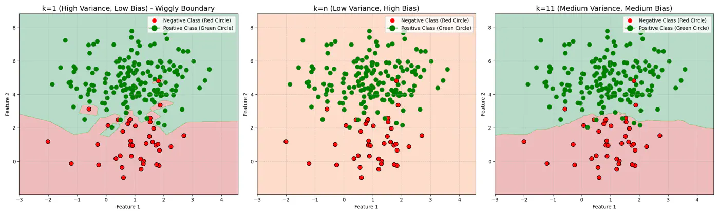
2.3.4 - Bias Variance Tradeoff
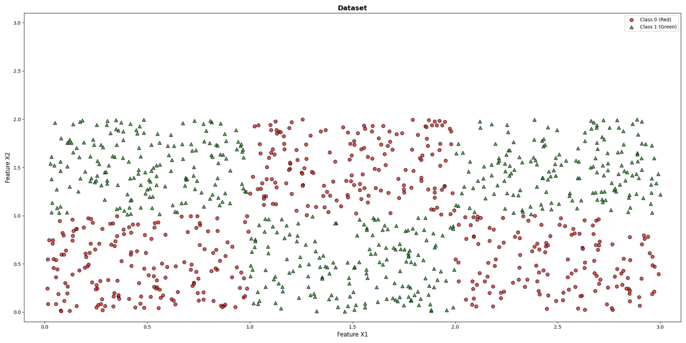
Let’s use this dataset to understand the impact of number of neighbours ‘k’.
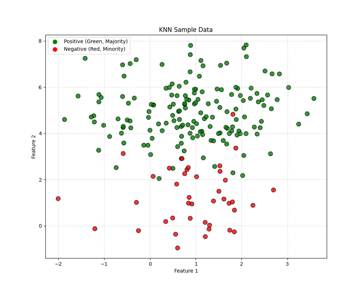
👉If ‘k’ is very large, say, k=n,
- model simply predicts the majority class of the entire dataset for every query point , i.e, under-fitting.
👉If ‘k’ is very small, say, k=1,
- model is highly sensitive to noise or outliers, as it looks at only 1 nearest neighbor, i.e, over-fitting.
Let’s plot Error vs ‘K’ neighbors:
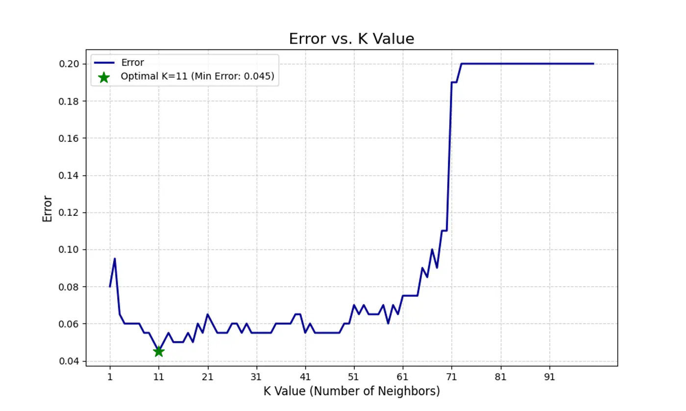
Figure 1: k=1, Over-fitting
Figure 2: k=n, Under-fitting
Figure 3: k=11, Lowest Error (Optimum)
End of Section
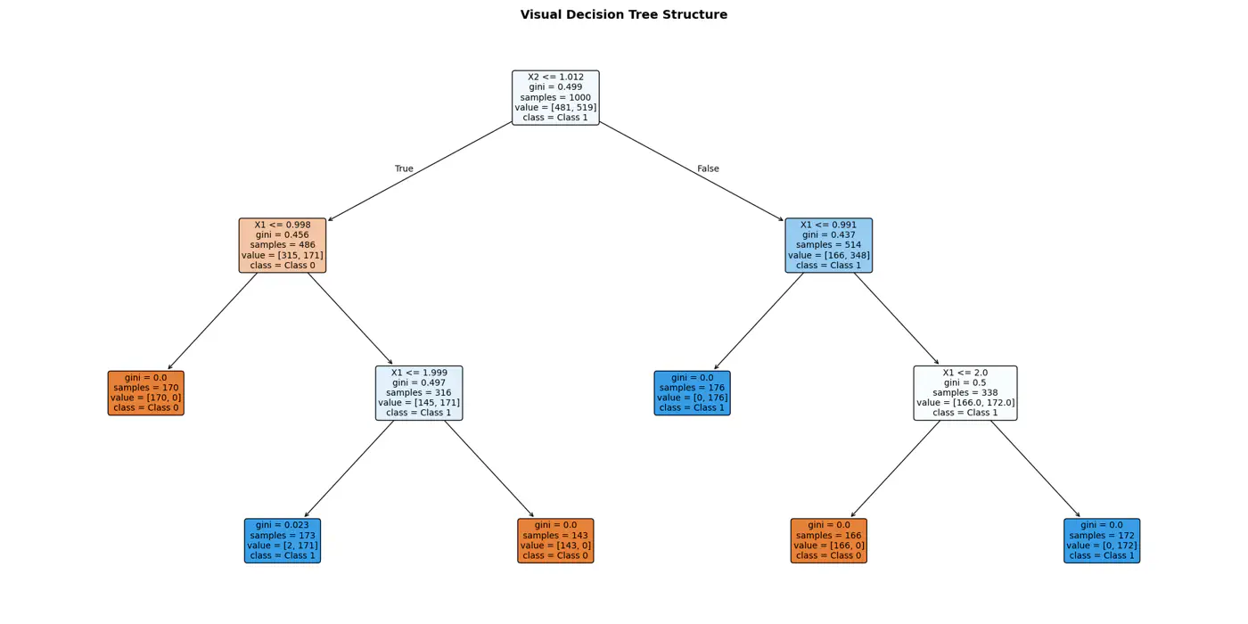
2.4.1 - Decision Trees Introduction
💡It can be written as nested 🕸️ if else statements.
e.g: To classify the left bottom corner red points we can write:
👉if (FeatureX1 <1 & FeatureX2 <1)
⭐️Extending the logic for all, we have an if else ladder like below:

👉Final decision boundaries will be something like below:
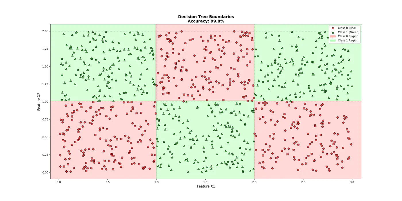
- Non-parametric model.
- Recursively partitions the feature space.
- Top-down, greedy approach to iteratively select feature splits.
- Maximize purity of a node, based on metrics, such as, Information Gain 💵 or Gini 🧞♂️Impurity.
Note: We can extract the if/else logic of the decision tree and write in C++/Java for better performance.
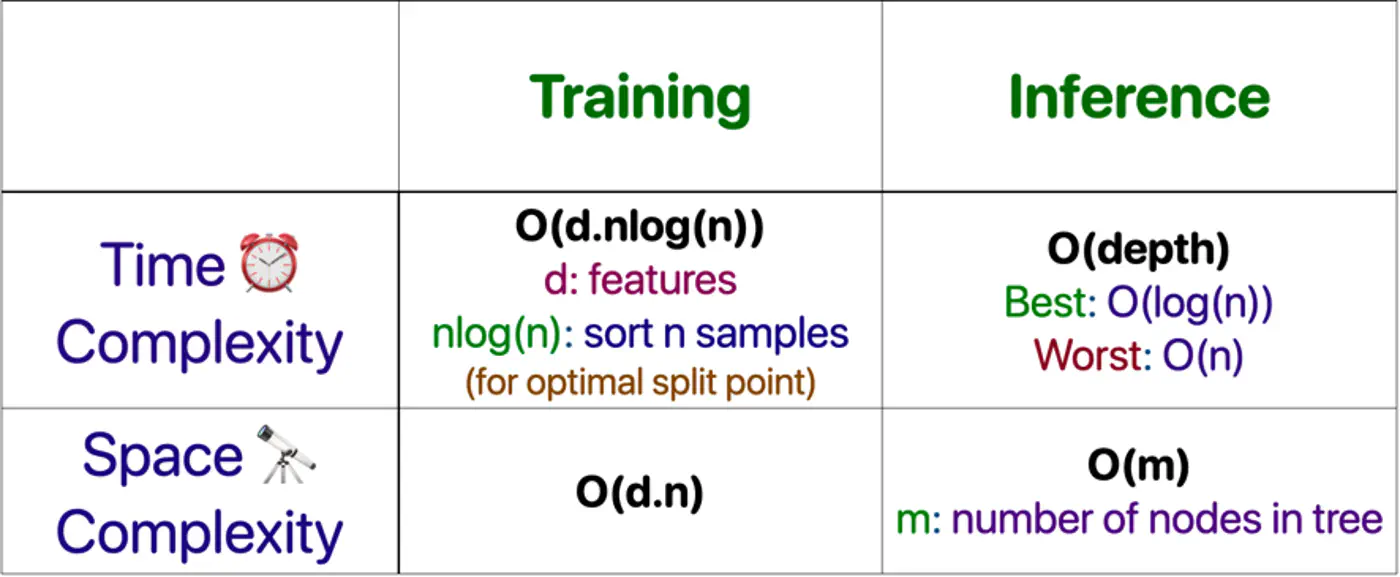
⭐️Building an optimal decision tree 🌲 is a NP-Hard problem.
👉(Time Complexity: Exponential; combinatorial search space)
- Pros
- No standardization of data needed.
- Highly interpretable.
- Good runtime performance.
- Works for both classification & regression.
- Cons
- Number of dimensions should not be too large. (Curse of dimensionality)
- Overfitting.
- As base learners in ensembles, such as, bagging(RF), boosting(GBDT), stacking, cascading, etc.
- As a baseline, interpretable, model or for quick feature selection.
- Runtime performance is important.
End of Section
2.4.2 - Purity Metrics
Decision trees recursively partition the data based on feature values.
Pure Leaf 🍃 Node: Terminal node where every single data point belongs to the same class.
💡Zero Uncertainty.
The goal of a decision tree algorithm is to find the split that maximizes information gain, meaning it removes the most uncertainty from the data.
So, what is information gain ?
How do we reduce uncertainty ?
Let’s understand few terms first, before we understand information gain.
Measure ⏱ of uncertainty, randomness, or impurity in a data.
\[H(S)=-\sum _{i=1}^{n}p_{i}\log(p_{i})\]Binary Entropy:
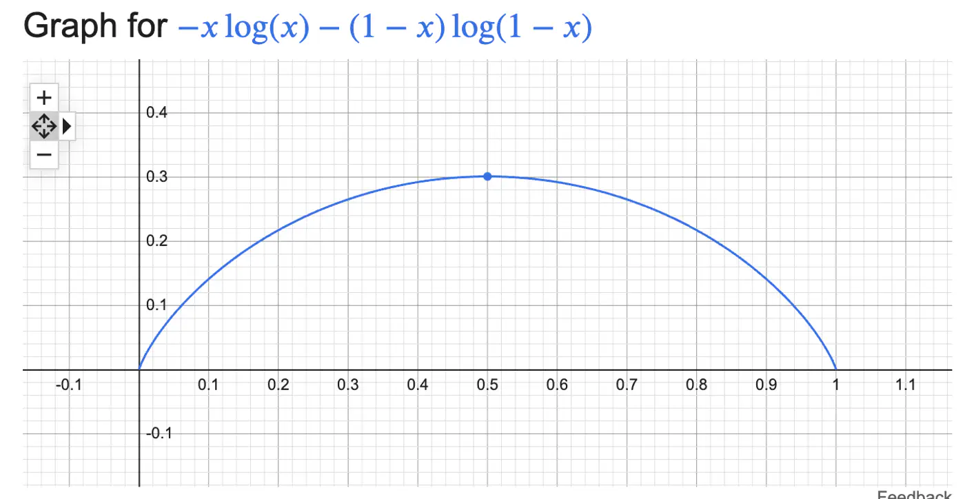
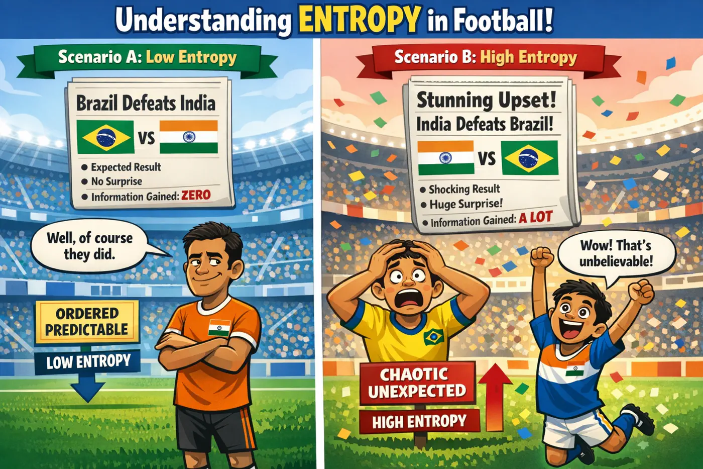
💡Entropy can also be viewed as the ‘average surprise'.
A highly certain event provides little information when it occurs (low surprise).
An unlikely event provides a lot of information (high surprise).
⭐️ Measures the reduction in entropy (uncertainty) achieved by splitting a dataset based on a specific attribute.
\[IG=Entropy(Parent)-\left[\frac{N_{left}}{N_{parent}}Entropy(Child_{left})+\frac{N_{right}}{N_{parent}}Entropy(Child_{right})\right] \]Note: The goal of a decision tree algorithm is to find the split that maximizes information gain, meaning it removes the most uncertainty from the data.
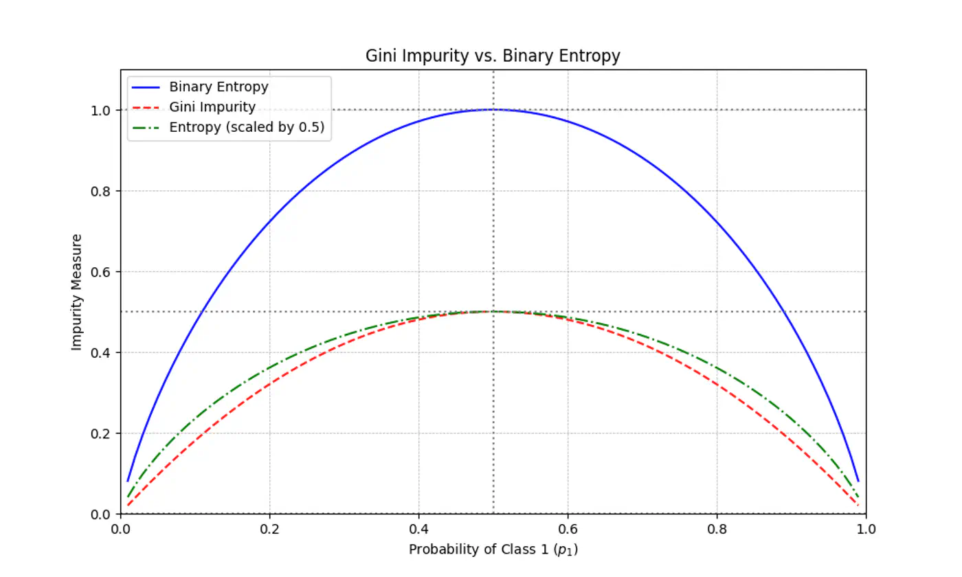
⭐️ Measures the probability of an element being incorrectly classified if it were randomly labeled according to the distribution of labels in a node.
\[Gini(S)=1-\sum_{i=1}^{n}(p_{i})^{2}\]- Range: 0 (Pure) - 0.5 (Maximum impurity)
Note: Gini is used in libraries like Scikit-Learn (as the default), because it avoids the computationally expensive 💰 log function.
Gini Impurity is a first-order approximation of Entropy.
For most of the real-world cases, choosing one over the other results in the exact same tree structure or negligible differences in accuracy.
When we plot the two functions, they follow nearly identical shapes.
End of Section
2.4.3 - Decision Trees For Regression
Decision Trees can also be used for Regression tasks but using a different metrics.
⭐️Metric:
- Mean Squared Error (MSE)
- Mean Absolute Error (MAE)
👉Say we have a following dataset, that we need to fit using decision trees:
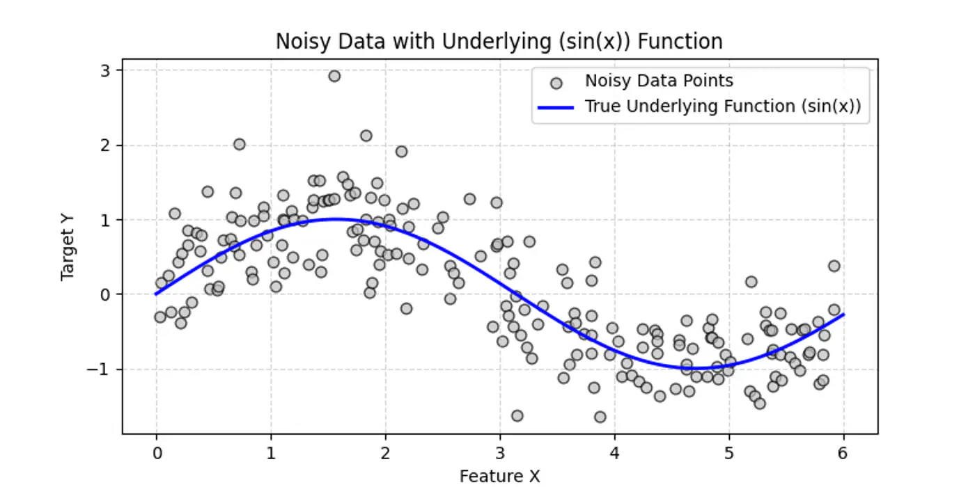
👉Decision trees try to find the decision splits, building step functions that approximate the actual curve, as shown below:
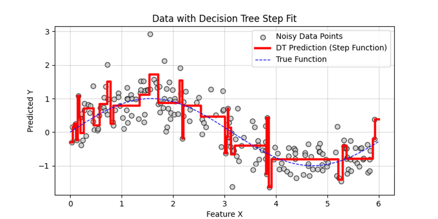
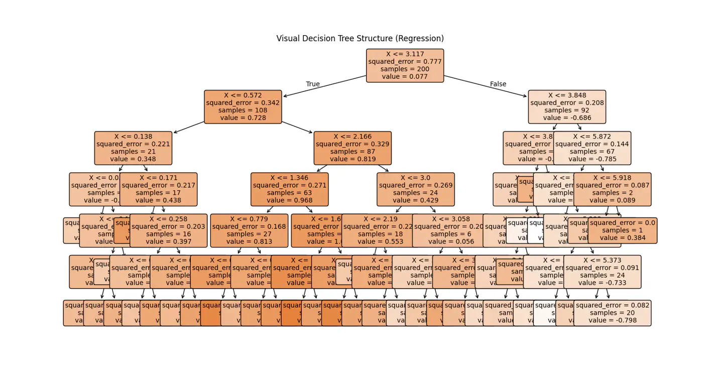
👉Internally the decision tree (if else ladder) looks like below:
Decision trees cannot predict values outside the range of the training data, i.e, extrapolation.
Let’s understand the interpolation and extrapolation cases one by one.
⭐️Predicting values within the range of features and targets observed during training 🏃♂️.
- Trees capture discontinuities perfectly, because they are piece-wise constant.
- They do not try to force a smooth line where a ‘jump’ exists in reality.
e.g: Predicting a house 🏡 price 💰 for a 3-BHK home when you have seen 2-BHK and 4-BHK homes in that same neighborhood.
⭐️Predicting values outside the range of training 🏃♂️data.
Problem:
Because a tree outputs the mean of training 🏃♂️ samples in a leaf, it cannot predict a value higher than the
highest ‘y’ it saw during training 🏃♂️.
- Flat-Line: Once a feature ‘X’ goes beyond the training boundaries, the tree falls into the same ‘last’ leaf forever.
e.g: Predicting the price 💰 of a house 🏡 in 2026 based on data from 2010 to 2025.
End of Section
2.4.4 - Regularization
- Pre-Pruning ✂️ &
- Post-Pruning ✂️
⭐️ ‘Early stopping’ heuristics (hyper-parameters).
- max_depth: Limits how many levels of ‘if else’ the tree can have; most common.
- min_samples_split: A node will only split, if it has at least ‘N’ samples; smooths the model (especially in regression), by ensuring predictions are based on an average of multiple points.
- max_leaf_nodes: Limiting the number of leaves reduces the overall complexity of the tree, making it simpler and less likely to memorize the training data’s noise.
- min_impurity_decrease: A split is only made if it reduces the impurity (Gini/MSE) by at least a certain threshold.
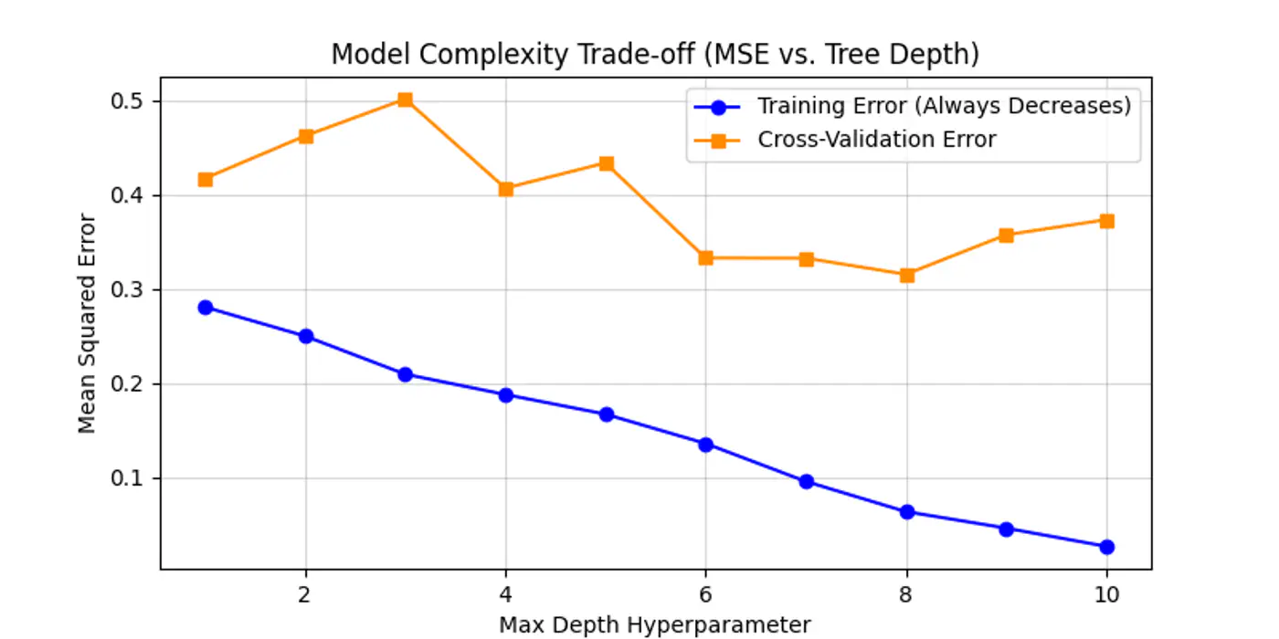
Below is an example for one of the hyper-parameter’s max_depth tuning.
As we can see below the cross-validation error decreases till depth=6 and after that reduction in error is not so significant.
Let the tree🌲 grow to its full depth (overfit) and then ‘collapse’ nodes that provide little predictive value.
Most common algorithm:
- Minimal Cost Complexity Pruning
💡Define a cost-complexity 💰 measure that penalizes the tree 🌲 for having too many leaves 🍃.
\[R_\alpha(T) = R(T) + \alpha |T|\]- R(T): total misclassification rate (or MSE) of the tree
- |T|: number of terminal nodes (leaves)
- \(\alpha\): complexity parameter (the ‘tax’ 💰 on complexity)
Logic:
- If \(\alpha\)=0, the tree is the original overfit tree.
- As \(\alpha\) increases 📈, the penalty for having many leaves grows 📈.
- To minimize the total cost 💰, the model is forced to prune branches that do not significantly reduce R(T).
- Use cross-validation to find the ‘sweet spot’ \(\alpha\) that minimizes validation error.
End of Section
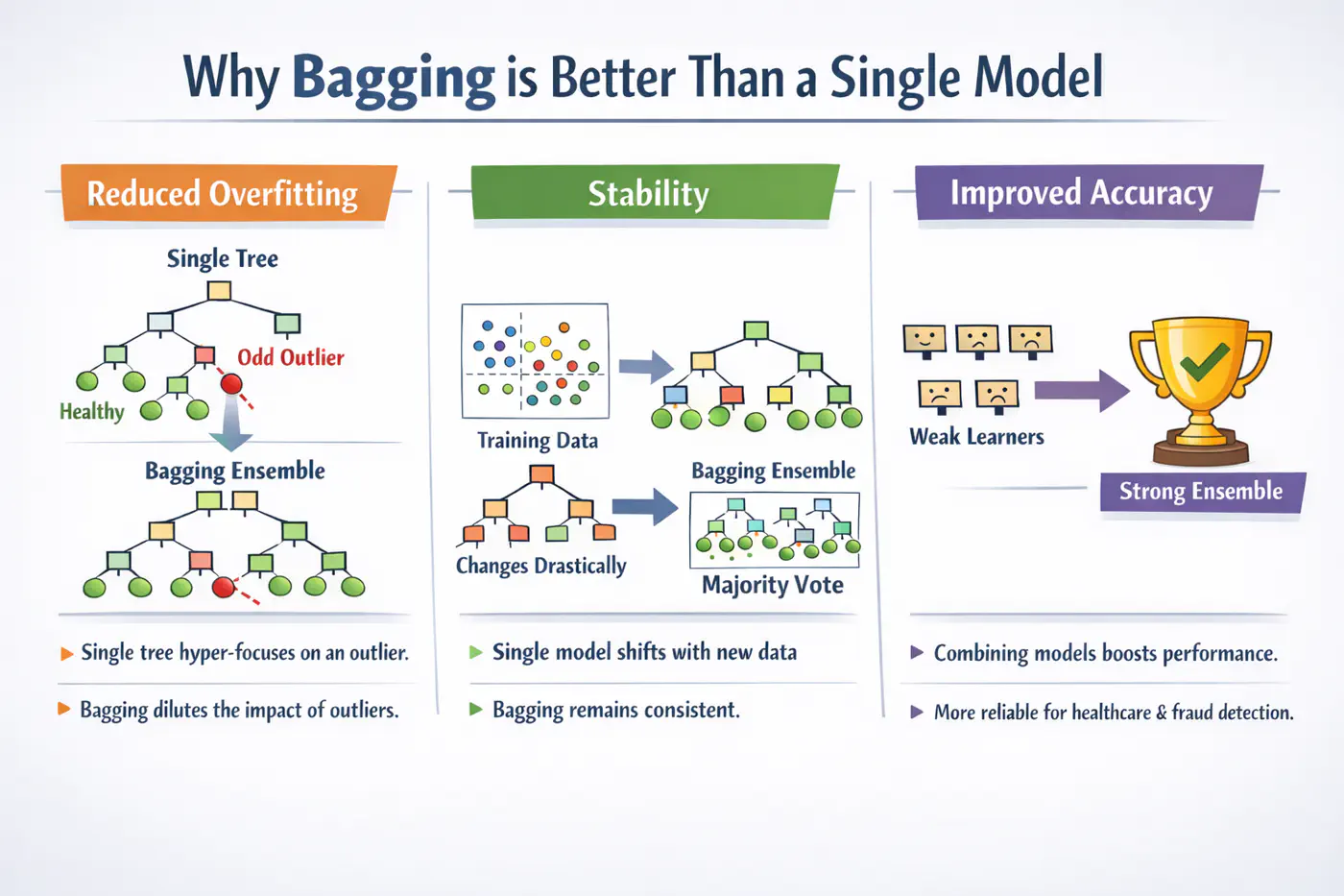
2.4.5 - Bagging
A single decision tree is highly sensitive to the specific training dataset.
Small changes, such as, a few different rows or the presence of an outlier, can lead to a completely different tree structure.Unpruned decision trees often grow until they perfectly classify the training set, essentially ‘memorizing’ noise and outliers, i.e, high variance, rather than finding general patterns.
Bagging = ‘Bootstrapped Aggregation’
Bagging 🎒is a parallel ensemble technique that reduces variance (without significantly increasing the bias) by training multiple versions of the same model on different random subsets of data and then combining their results.
Note: Bagging uses deep trees (overfit) and combines them to reduce variance.
Bootstrapping = ‘Without external help’
Given a training 🏃♂️set D of size ’n’, we create B new training sets D by sampling ’n’ observations from D ‘with replacement'.
💡Since, we are sampling ‘with replacement’, so, some data points may be picked multiple times, while others may not be picked at all.
- The probability that a specific observation is not selected in a bootstrap sample of size ’n’ is: \[\lim_{n \to \infty} \left(1 - \frac{1}{n}\right)^n = \frac{1}{e} \approx 0.368\]
🧐This means each tree is trained on roughly 63.2% of the unique data, while the remaining 36.8% (the Out-of-Bag or OOB set) can be used for cross validation.
⭐️Say we train ‘B’ models (base-learners), each with variance \(\sigma^2\) .
👉Average variance of ‘B’ models (trees) if all are independent:
\[Var(X)=\frac{\sigma^{2}}{B}\]👉Since, bootstrap samples are derived from the same dataset, the trees are correlated with some correlation coefficient ‘\(\rho\)'.
So, the true variance of bagged ensemble is:
\[Var(f_{bag}) = \rho \sigma^2 + \frac{1-\rho}{B} \sigma^2\]- \(\rho\)= 0; independent models, most reduction in variance.
- \(\rho\)= 1; fully correlated models, no improvement in variance.
- 0<\(\rho\)<1; As correlation decreases, variance reduces .
End of Section
2.4.6 - Random Forest
💡If one feature is extremely predictive (e.g., ‘Area’ for house prices), almost every bootstrap tree will split on that feature at the root.
👉This makes the trees(models) very similar, leading to a high correlation ‘\(\rho\)’.
\[Var(f_{bagging})=ρ\sigma^{2}+\frac{1-ρ}{B}\sigma^{2}\]💡Choose a random subset of ‘m’ features from the total ‘d’ features, reducing the correlation ‘\(\rho\)’ between trees.
👉By forcing trees to split on ‘sub-optimal’ features, we intentionally increase the variance of individual trees; also the bias is slightly increased (simpler trees).
Standard heuristics:
- Classification: \(m = \sqrt{d}\)
- Regression: \(m = \frac{d}{3}\)
💡Because ‘\(\rho\)’ is the dominant factor in the variance of the ensemble when B is large, the overall ensemble variance Var(\(f_{rf}\)) drops significantly lower than standard Bagging.
\[Var(f_{rf})=ρ\sigma^{2}+\frac{1-ρ}{B}\sigma^{2}\]💡A Random Forest will never overfit by adding more trees (B).
It only converges to the limit: ‘\(\rho\sigma^2\)’.
Overfitting is controlled by:
- depth of the individual trees.
- size of the feature subset ‘m'.
- High Dimensionality: 100s or 1000s of features; RF’s feature sampling prevents a few features from masking others.
- Tabular Data (with Complex Interactions): Captures non-linear relationships without needing manual feature engineering.
- Noisy Datasets: The averaging process makes RF robust to outliers (especially if using min_samples_leaf).
- Automatic Validation: Need a quick estimate of generalization error without doing 10-fold CV (via OOB Error).
End of Section
2.4.7 - Extra Trees
💡In a standard Decision Tree or Random Forest, the algorithm searches for the optimal split point (the threshold ’s’) that maximizes Information Gain or minimizes MSE.
👉This search is:
- computationally expensive (sort + mid-point) and
- tends to follow the noise in the training 🏃♂️data.
Adding randomness (right kind) in ensemble averaging reduces correlation/variance.
\[Var(f_{bag})=ρ\sigma^{2}+\frac{1-ρ}{B}\sigma^{2}\]- Random Thresholds: Instead of searching for the best split point (computationally expensive 💰) for a feature, it picks a threshold at random from a uniform distribution between the feature’s local minimum and maximum.
- Entire Dataset: Uses entire training dataset (default) for every tree; no bootstrapping.
- Random Feature Subsets: Random subset of m<n features is used in each decision tree.
Picking thresholds randomly has two effects:
- Structural correlation between trees becomes extremely low.
- Individual trees are ‘weaker’ and have higher bias than a standard optimized tree.
👉The massive drop in ‘\(\rho\)’ often outweighs the slight increase in bias, leading to an overall ensemble that is smoother and more robust to noise than a standard Random Forest.
Note: Extra Trees are almost always grown to full depth, as they may need extra splits to find the same decision boundary.
- Performance: Significantly faster to train, as it does not sort data to find optimal split.
Note: If we are working with billions of rows or thousands of features, ET can be 3x to 5x faster than a Random Forest(RF). - Robustness to Noise: By picking thresholds randomly, tends to ‘handle’ the noise more effectively than RF.
- Feature Importance: Because ET is so randomized, it often provides more ‘stable’ feature importance scores.
Note: It is less likely to favor a high-cardinality feature (e.g. zip-code) just because it has more potential split points.
End of Section
2.4.8 - Boosting
⭐️In Bagging 🎒we trained multiple strong(over-fit, high variance) models (in parallel) and then averaged them out to reduce variance.
💡Similarly, we can train many weak(under-fit, high bias) models sequentially, such that, each new model corrects the errors of the previous ones to reduce bias.
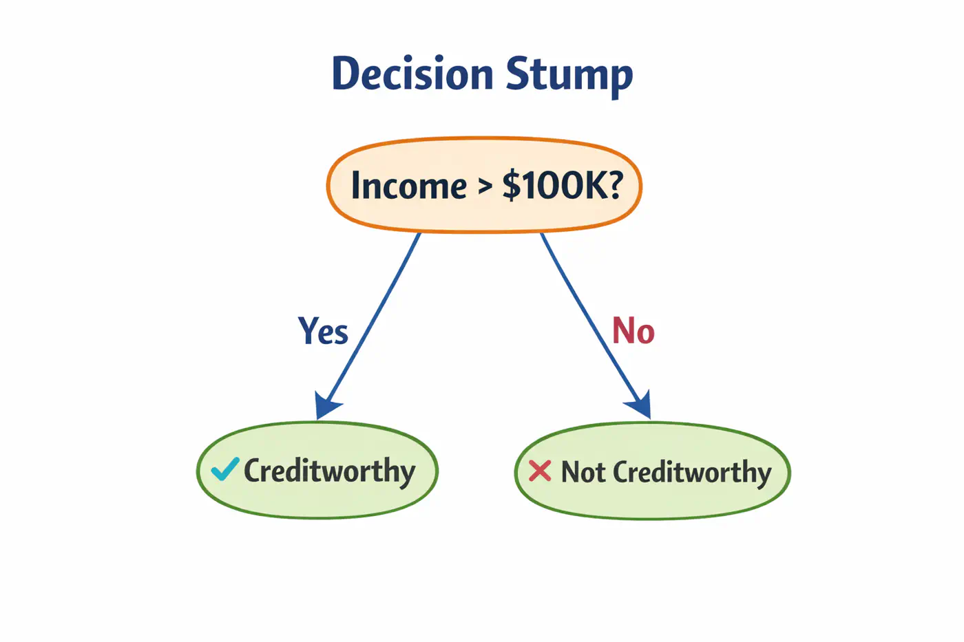
⚔️ An ensemble learning approach where multiple ‘weak learners’ (typically simple models like shallow decision trees 🌲 or ‘stumps’) are sequentially combined to create a single strong predictive model.
⭐️The core principle is that each subsequent model focuses 🎧 on correcting the errors made by its predecessors.
- AdaBoost(Adaptive Boosting)
- Gradient Boosting Machine (GBM)
- XGBoost
- LightGBM (Microsoft)
- CatBoost (Yandex)
End of Section
2.4.9 - AdaBoost
💡Works by increasing 📈 the weight 🏋️♀️ of misclassified data points after each iteration, forcing the next weak learner to ‘pay more attention’🚨 to the difficult cases.
⭐️ Commonly used for classification.
👉Weak learners are typically ‘Decision Stumps’, i.e, decision trees🌲with a depth of only one (1 split, 2 leaves 🍃).
- Assign an equal weight 🏋️♀️to every data point; \(w_i = 1/n\), where ’n’=number of samples.
- Build a decision stump that minimizes the weighted classification error.
- Calculate total error; \(E_m = \Sigma w_i\).
- Determine ‘amount of say’, i.e, the weight 🏋️♀️ of each stump in final decision.
\[\alpha_m = \frac{1}{2}ln\left( \frac{1-E_m}{E_m} \right)\]
- Low error results in a high positive \(\alpha\) (high influence).
- 50% error (random guessing) results in an \(\alpha = 0\) (no influence).
- Update sample weights 🏋️♀️.
- Misclassified samples: Weight 🏋️♀️ increases by \(e^{\alpha_m}\).
- Correctly classified samples: Weight 🏋️♀️ decreases by \(e^{-\alpha_m}\).
- Normalization: All new weights 🏋️♀️ are divided by their total sum so they add up back to 1.
- Iterate for a specified number of estimators (n_estimators).
👉 To classify a new data point, every stump makes a prediction (+1 or -1).
These are multiplied by their respective ‘amount of say’ \(\alpha_m\) and summed.
\[H(x)=sign\sum_{m=1}^{M}\alpha_{m}⋅h_{m}(x)\]👉 If the total weighted 🏋️♀️ sum is positive, the final class is +1; otherwise -1.
Note: Sensitive to outliers; Because AdaBoost aggressively increases weights 🏋️♀️ on misclassified points, it may ‘over-focus’ on noisy outliers, hurting performance.
End of Section
2.4.10 - Gradient Boosting Machine
GBM treats the final model \(F_m(x)\) as weighted 🏋️♀️ sum of ‘m’ weak learners:
\[ F_{M}(x)=\underbrace{F_{0}(x)}_{\text{Initial\ Guess}}+\nu \sum _{m=1}^{M}\underbrace{\left(\sum _{j=1}^{J_{m}}\gamma _{jm}\mathbb{I}(x\in R_{jm})\right)}_{\text{Weak\ Learner\ }h_{m}(x)}\]- \(F_0(x)\): The initial base model (usually a constant).
- M: The total number of boosting iterations (number of trees).
- \(\gamma_{jm}\)(Leaf Weight): The optimized value for leaf in tree .
- \(\nu\)(Nu): The Learning Rate or Shrinkage; prevent overfitting.
- \(\mathbb{I}(x\in R_{jm})\): ‘Indicator Function’; It is 1 if data point falls into leaf of the tree, and 0 otherwise.
- \(R_{jm}\)(Regions): Region of \(j_{th}\) leaf in \(m_{th}\)tree.
📍In Gradient Descent, we update parameters ‘\(\Theta\)';
📍In GBM, we update the predictions F(x) themselves.
🦕We move the predictions in the direction of the negative gradient of the loss function L(y, F(x)).
🎯We want to minimize loss:
\[\mathcal{L}(F) = \sum_{i=1}^n L(y_i, F(x_i))\]✅ In parameter optimization we update weights 🏋️♀️:
\[w_{t+1} = w_t - \eta \cdot \nabla_{w}\mathcal{L}(w_t)\]✅ In gradient boosting, we update the prediction function:
\[F_m(x) = F_{m-1}(x) -\eta \cdot \nabla_F \mathcal{L}(F_{m-1}(x))\]➡️ The gradient is calculated w.r.t. predictions, not weights.
In GBM we can use any loss function as long as it is differentiable, such as, MSE, log loss, etc.
Loss(MSE) = \((y_i - F_m(x_i))^2\)
\[\frac{\partial L}{F_m(x_i)} = -2 (y-F_m(x_i))\]\[\implies \frac{\partial L}{F_m(x_i)} \propto - (y-F_m(x_i))\]👉Pseudo Residual (Error) = - Gradient
💡To minimize loss, take derivative of loss function w.r.t ‘\(\gamma\)’ and equate to 0:
\[F_0(x) = \arg\min_{\gamma} \sum_{i=1}^n L(y_i, \gamma)\]MSE Loss = \(\mathcal{L}(y_i, \gamma) = \sum_{i=1}^n(y_i -\gamma)^2\)
\[ \begin{aligned} &\frac{\partial \mathcal{L}(y_i, \gamma)}{\partial \gamma} = -2 \cdot \sum_{i=1}^n(y_i -\gamma) = 0 \\ &\implies \sum_{i=1}^n (y_i -\gamma) = 0 \\ &\implies \sum_{i=1}^n y_i = n.\gamma \\ &\therefore \gamma = \frac{1}{n} \sum_{i=1}^n y_i \end{aligned} \]💡To minimize cost, take derivative of cost function w.r.t ‘\(\gamma\)’ and equate to 0:
Cost Function = \(J(\gamma )\)
\[J(\gamma )=\sum _{x_{i}\in R_{jm}}\frac{1}{2}(y_{i}-(F_{m-1}(x_{i})+\gamma ))^{2}\]We know that:
\[ r_{i}=y_{i}-F_{m-1}(x_{i})\]\[\implies J(\gamma )=\sum _{x_{i}\in R_{jm}}\frac{1}{2}(r_{i}-\gamma )^{2}\]\[\frac{d}{d\gamma }\sum _{x_{i}\in R_{jm}}\frac{1}{2}(r_{i}-\gamma )^{2}=\sum _{x_{i}\in R_{jm}}-(r_{i}-\gamma )=0\]\[\implies \sum _{x_{i}\in R_{jm}}\gamma -\sum _{x_{i}\in R_{jm}}r_{i}=0\]👉Since, \(\gamma\) is constant for all \(n_j\) samples in the leaf, \(\sum _{x_{i}\in R_{jm}}\gamma =n_{j}\gamma \)
\[n_{j}\gamma =\sum _{x_{i}\in R_{jm}}r_{i}\]\[\implies \gamma =\frac{\sum _{x_{i}\in R_{jm}}r_{i}}{n_{j}}\]Therefore, \(\gamma\) = average of all residuals in the leaf.
Note: \(R_{jm}\)(Regions): Region of \(j_{th}\) leaf in \(m_{th}\)tree.
End of Section
2.4.11 - GBDT Algorithm
Gradient Boosted Decision Tree (GBDT) is a decision tree based implementation of Gradient Boosting Machine (GBM).
GBM treats the final model \(F_m(x)\) as weighted 🏋️♀️ sum of ‘m’ weak learners (decision trees):
\[ F_{M}(x)=\underbrace{F_{0}(x)}_{\text{Initial\ Guess}}+\nu \sum _{m=1}^{M}\underbrace{\left(\sum _{j=1}^{J_{m}}\gamma _{jm}\mathbb{I}(x\in R_{jm})\right)}_{\text{Decision\ Tree\ }h_{m}(x)}\]- \(F_0(x)\): The initial base model (usually a constant).
- M: The total number of boosting iterations (number of trees).
- \(\gamma_{jm}\)(Leaf Weight): The optimized value for leaf in tree .
- \(\nu\)(Nu): The Learning Rate or Shrinkage; prevent overfitting.
- \(\mathbb{I}(x\in R_{jm})\): ‘Indicator Function’; It is 1 if data point falls into leaf of the tree, and 0 otherwise.
- \(R_{jm}\)(Regions): Region of \(j_{th}\) leaf in \(m_{th}\)tree.
- Step 1: Initialization.
- Step 2: Iterative loop 🔁 : for i=1 to m.
- 2.1: Calculate pseudo residuals ‘\(r_{im}\)'.
- 2.2: Fit a regression tree 🌲‘\(h_m(x)\)'.
- 2.3:Compute leaf 🍃weights 🏋️♀️ ‘\(\gamma_{jm}\)'.
- 2.4:Update the model.
Start with a function that minimizes our loss function;
for MSE its mean.
MSE Loss = \(\mathcal{L}(y_i, \gamma) = \sum_{i=1}^n(y_i -\gamma)^2\)
Find the ‘gradient’ of error;
Tells us the direction and magnitude needed to reduce the loss.
Train a tree to predict the residuals ‘\(h_m(x)\)';
- Tree 🌲 partitions the data into leaves 🍃 (\(R_{jm}\)regions )
Within each leaf 🍃, we calculate the optimal value ‘\(\gamma_{jm}\)’ that minimizes the loss for the samples in that leaf 🍃.
\[\gamma_{jm} = \arg\min_{\gamma} \sum_{x_i \in R_{jm}} L(y_i, F_{m-1}(x_i) + \gamma)\]➡️ The optimal leaf 🍃value is the ‘Mean’(MSE) of the residuals; \(\gamma = \frac{\sum r_i}{n_j}\)
Add the new ‘correction’ to the existing model, scaled by the learning rate.
\[F_{m}(x)=F_{m-1}(x)+\nu \cdot \underbrace{\sum _{j=1}^{J_{m}}\gamma _{jm}\mathbb{I}(x\in R_{jm})}_{h_{m}(x)}\]- \(\mathbb{I}(x\in R_{jm})\): ‘Indicator Function’; It is 1 if data point falls into leaf of the tree, and 0 otherwise.
End of Section
2.4.12 - GBDT Example
Gradient Boosted Decision Tree (GBDT) is a decision tree based implementation of Gradient Boosting Machine (GBM).
GBM treats the final model \(F_m(x)\) as weighted 🏋️♀️ sum of ‘m’ weak learners (decision trees):
\[ F_{M}(x)=\underbrace{F_{0}(x)}_{\text{Initial\ Guess}}+\nu \sum _{m=1}^{M}\underbrace{\left(\sum _{j=1}^{J_{m}}\gamma _{jm}\mathbb{I}(x\in R_{jm})\right)}_{\text{Decision\ Tree\ }h_{m}(x)}\]- \(F_0(x)\): The initial base model (usually a constant).
- M: The total number of boosting iterations (number of trees).
- \(\gamma_{jm}\)(Leaf Weight): The optimized value for leaf in tree .
- \(\nu\)(Nu): The Learning Rate or Shrinkage; prevent overfitting.
- \(\mathbb{I}(x\in R_{jm})\): ‘Indicator Function’; It is 1 if data point falls into leaf of the tree, and 0 otherwise.
- \(R_{jm}\)(Regions): Region of \(j_{th}\) leaf in \(m_{th}\)tree.
- Step 1: Initialization.
- Step 2: Iterative loop 🔁 : for i=1 to m.
- 2.1: Calculate pseudo residuals ‘\(r_{im}\)'.
- 2.2: Fit a regression tree 🌲‘\(h_m(x)\)'.
- 2.3:Compute leaf 🍃weights 🏋️♀️ ‘\(\gamma_{jm}\)'.
- 2.4:Update the model.
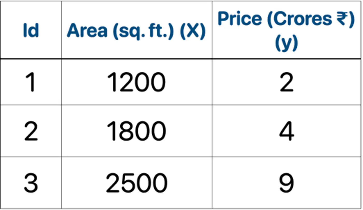
👉Loss = MSE, Learning rate (\(\nu\)) = 0.5
- Initialization : \(F_0(x) = mean(2,4,9) = 5.0\)
- Iteration 1(m=1):
2.1: Calculate residuals ‘\(r_{i1}\)'
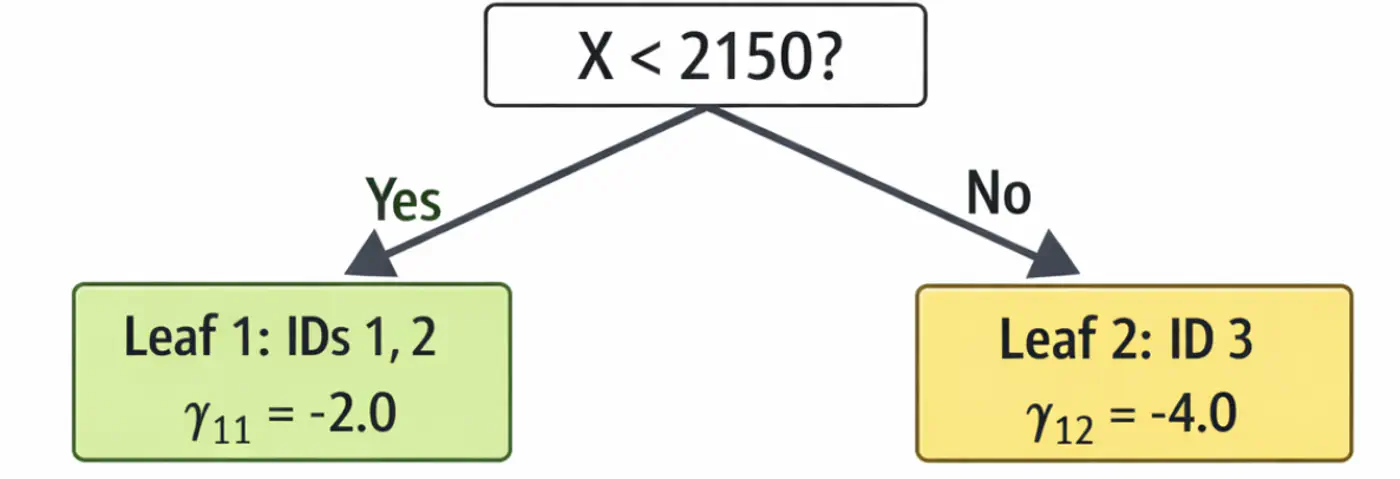
\[\begin{aligned} r_{11} &= 2-5 = -3.0 \\ r_{21} &= 4-5 = -1.0 \\ r_{31} &= 9-5 = 4.0 \\ \end{aligned} \]2.2: Fit tree(\(h_1\)); Split at X<2150 (midpoint of 1800 and 2500)
2.3: Compute leaf weights \(\gamma_{j1}\)
- Y-> Leaf 1: Ids 1, 2 ( \(\gamma_{11}\)= -2.0)
- N-> Leaf 2: Id 3 ( \(\gamma_{21}\)= 4.0)
2.4: Update predictions (\(F_1 = F_0 + 0.5 \cdot \gamma\))
\[ \begin{aligned} F_1(x_1) &= 5.0 + 0.5(-2.0) = \mathbf{4.0}\ \\F_1(x_2) &= 5.0 + 0.5(-2.0) = \mathbf{4.0}\ \\F_1(x_3) &= 5.0 + 0.5(4.0) = \mathbf{7.0}\ \\ \end{aligned} \]Tree 1:
- Iteration 2(m=2):
2.1: Calculate residuals ‘\(r_{i2}\)'
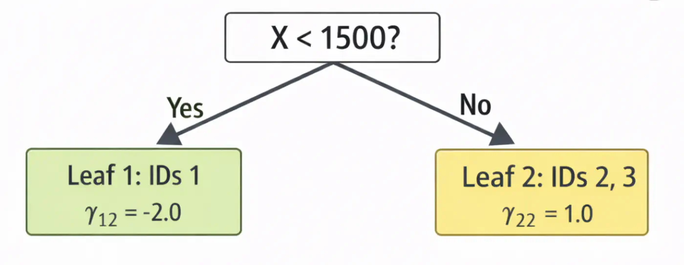
\[ \begin{aligned} r_{12} &= 2-4.0 = -2.0 \\ r_{22} &= 4-4.0 = 0.0 \\ r_{32} &= 9-7.0 = 2.0 \\ \end{aligned} \]2.2: Fit tree(\(h_2\)); Split at X<1500 (midpoint of 1200 and 1800)
2.3: Compute leaf weights \(\gamma_{j2}\)
- Y-> Leaf 1: Ids 1 ( \(\gamma_{12}\)= -2.0)
- N-> Leaf 2: Id 2, 3 ( \(\gamma_{22}\)= 1.0)
2.4: Update predictions (\(F_1 = F_0 + 0.5 \cdot \gamma\))
\[ \begin{aligned} F_2(x_1) &= 4.0 + 0.5(-2.0) = \mathbf{3.0} \\F_2(x_2) &= 4.0 + 0.5(1.0) = \mathbf{4.5} \\ F_2(x_3) &= 7.0 + 0.5(1.0) = \mathbf{7.5}\ \\ \end{aligned} \]Tree 2:
Note: We can keep adding more trees with every iteration;
ideally, learning rate \(\nu\) is small, say 0.1, so that we do not overshoot and converge slowly.
Let’s predict the price of a house with area = 2000 sq. ft.
- \(F_{0}=5.0\)
- Pass though tree 1 (\(h_1\)): is 2000 < 2150 ? Yes, \(\gamma_{11}\)= -2.0
- Contribution (\(h_1\)) = 0.5 x (-2.0) = -1.0
- Pass though tree 2 (\(h_2\)): is 2000 < 1500 ? No, \(\gamma_{22}\) = 1.0
- Contribution(\(h_2\)) = 0.5 x (1.0) = 0.5
- Final prediction = 5.0 - 1.0 + 0.5 = 4.5
Therefore, the price of a house with area = 2000 sq. ft is Rs 4.5 crores, which is very close.
In just 2 iterations, although with higher learning rate (\(\nu=0.5\)), we were able to get a fairly good estimate.
End of Section
2.4.13 - Advanced GBDT Algorithms
🔵 LightGBM (Light Gradient Boosting Machine)
⚫️ CatBoost (Categorical Boosting)
⭐️An optimized and highly efficient implementation of gradient boosting.
👉 Widely used in competitive data science (like Kaggle) due to its speed and performance.
Note: Research project developed by Tianqi Chen during his doctoral studies at the University of Washington.
⭐️Developed by Microsoft, this framework is designed for high speed and efficiency with large datasets.
👉It grows trees leaf-wise rather than level-wise and uses Gradient-based One-Side Sampling (GOSS) to speed 🐇 up the finding of optimal split points.
End of Section
2.4.14 - XgBoost
⭐️An optimized and highly efficient implementation of gradient boosting.
👉 Widely used in competitive data science (like Kaggle) due to its speed and performance.
Note: Research project developed by Tianqi Chen during his doctoral studies at the University of Washington.
🔵 Regularization
🔵 Sparsity-Aware Split Finding
⭐️Uses second derivative (Hessian), i.e, curvature, in addition to first derivative (gradient) to optimize the objective function more quickly and accurately than GBDT.
Let’s understand this with the problem to minimize \(f(x) = x^4\), using:
Gradient descent (uses only 1st order derivative, \(f'(x) = 4x^3\))
Newton’s method (uses both 1st and 2nd order derivatives \(f''(x) = 12x^2\))

- Adds explicit regularization terms (L1/L2 on leaf weights and tree complexity) into the boosting objective, helping reduce over-fitting. \[ \text{Objective} = \underbrace{\sum_{i=1}^{n} L(y_i, \hat{y}_i)}_{\text{Training Loss}} + \underbrace{\gamma T + \frac{1}{2}\lambda \sum_{j=1}^{T} w_j^2 + \alpha \sum_{j=1}^{T} |w_j|}_{\text{Regularization (The Tax)}} \]
💡Real-world data often contains many missing values or zero-entries (sparse data).
👉 XGBoost introduces a ‘default direction’ for each node.
➡️During training, it learns the best direction (left or right) for missing values to go, making it significantly faster and more robust when dealing with sparse or missing data.
End of Section
2.4.15 - LightGBM
⭐️Developed by Microsoft, this framework is designed for high speed and efficiency with large datasets.
👉It grows trees leaf-wise rather than level-wise and uses Gradient-based One-Side Sampling (GOSS) to speed 🐇 up the finding of optimal split points.
🔵 Exclusive Feature Bundling (EFB)
🔵 Leaf-wise Tree Growth Strategy
- ❌ Traditional GBDT uses all data instances for gradient calculation, which is inefficient.
- ✅ GOSS focuses 🔬on instances with larger gradients (those that are less well-learned or have higher error).
- 🐛 Keeps all instances with large gradients but randomly samples from those with small gradients.
- 🦩This way, it prioritizes the most informative examples for training, significantly reducing the data used and speeding up 🐇 the process while maintaining accuracy.
- 🦀 High-dimensional data often contains many sparse, mutually exclusive features (features that never take a non-zero value simultaneously, such as, One Hot Encoding (OHE)).
- 💡 EFB bundles the non-overlapping features into a single, dense feature, reducing the number of features, without losing much information, saving computation.
- ❌ Traditional gradient boosting machines (like XGBoost), the trees are built level-wise (BFS-like), meaning all nodes at the current level are split before moving to the next level.
- ✅ LightGBM maintains a set of all potential leaves that can be split at any given time and selects the leaf (for splitting) that provides the maximum gain across the entire tree, regardless of its depth.
Note: Need mechanisms to avoid over-fitting.
End of Section
2.4.16 - CatBoost
🔵 Symmetric(Oblivious) Trees
🔵 Handling Missing Values
- ❌ Standard target encoding can lead to target leakage, where the model uses information from the target variable during training that would not be available during inference.
👉(model ‘cheats’ by using a row’s own label to predict itself). - ✅ CatBoost calculates the target statistics (average target value) for each category based only on the history of previous training examples in a random permutation of the data.
🦋 Uses symmetric decision trees by default.
👉 In symmetric trees, the same split condition is applied at each level across the entire tree structure.🦘Does not walk down the tree using ‘if-else’ logic, instead it evaluates decision conditions to create a binary index (e.g 101) and jumps directly to that leaf 🍃 in memory 🧠.
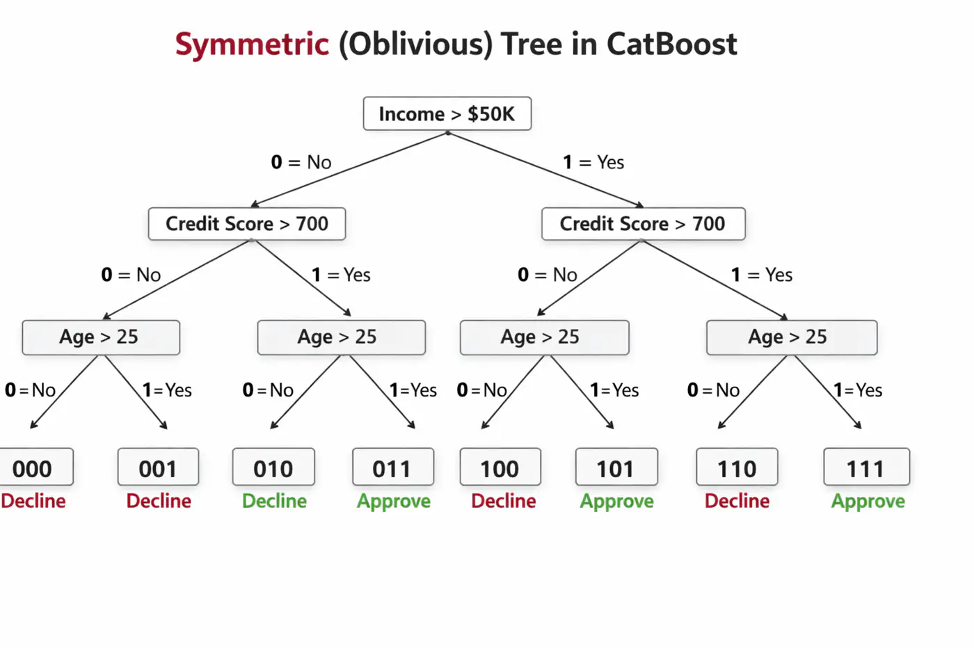
⚙️ CatBoost offers built-in, intelligent handling of missing values and sparse features, which often require manual preprocessing in other GBDT libraries.
💡Treats ‘NaN’ as a distinct category, reducing the need for imputation.
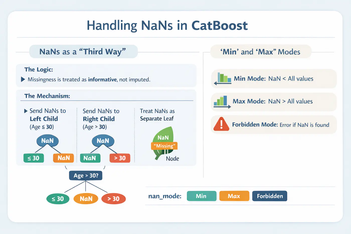
End of Section
2.5.1 - SVM Intro
⭐️We have two classes of points (e.g. Cats 😸vs. Dogs 🐶) that can be separated by a straight line.
👉 Many such lines exist !
💡SVM asks: “Which line is the safest?”
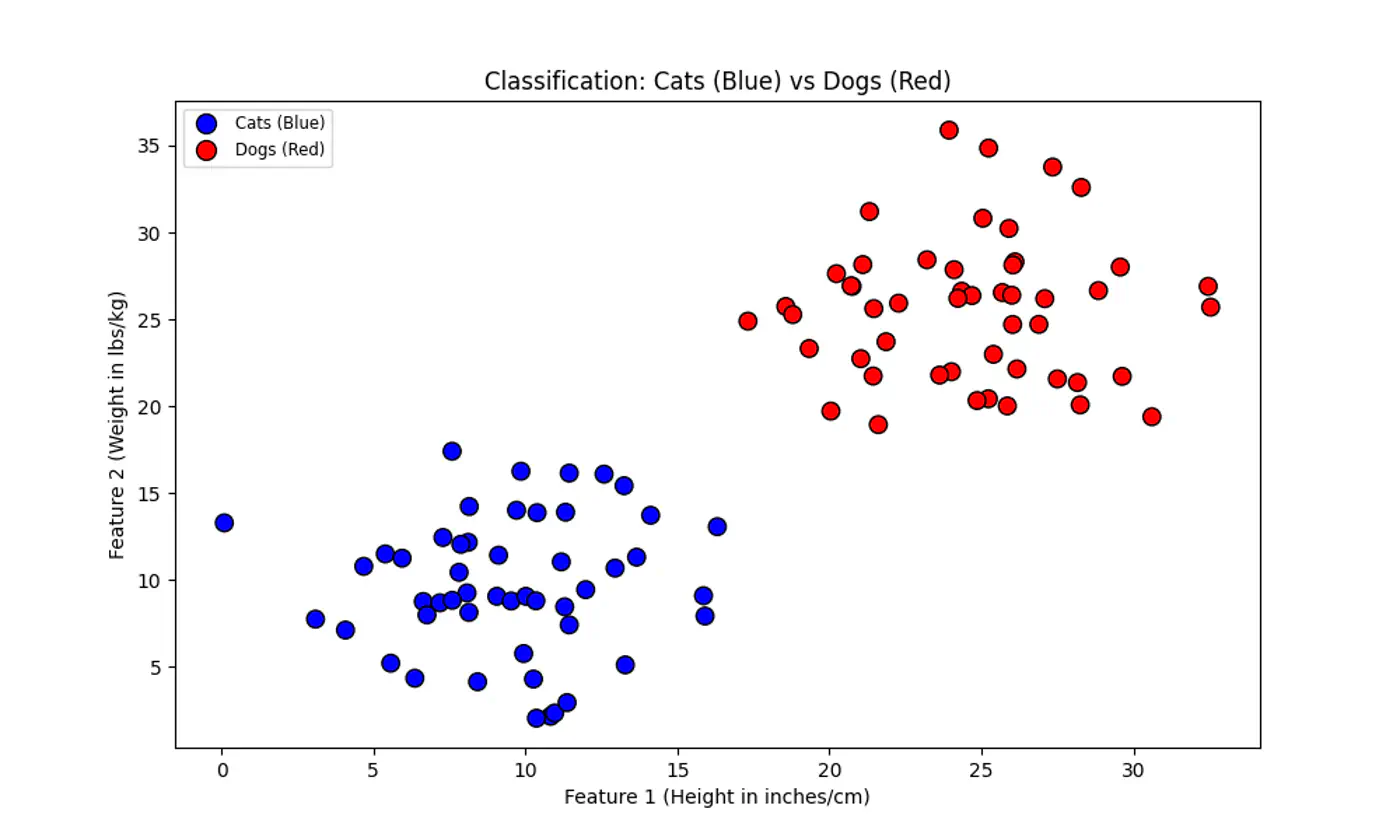
💡Think of the decision boundary as the center-line of a highway 🛣️.
SVM tries to make this highway 🛣️ as wide as possible without hitting any ‘buildings’ 🏡 (data points) on either side.
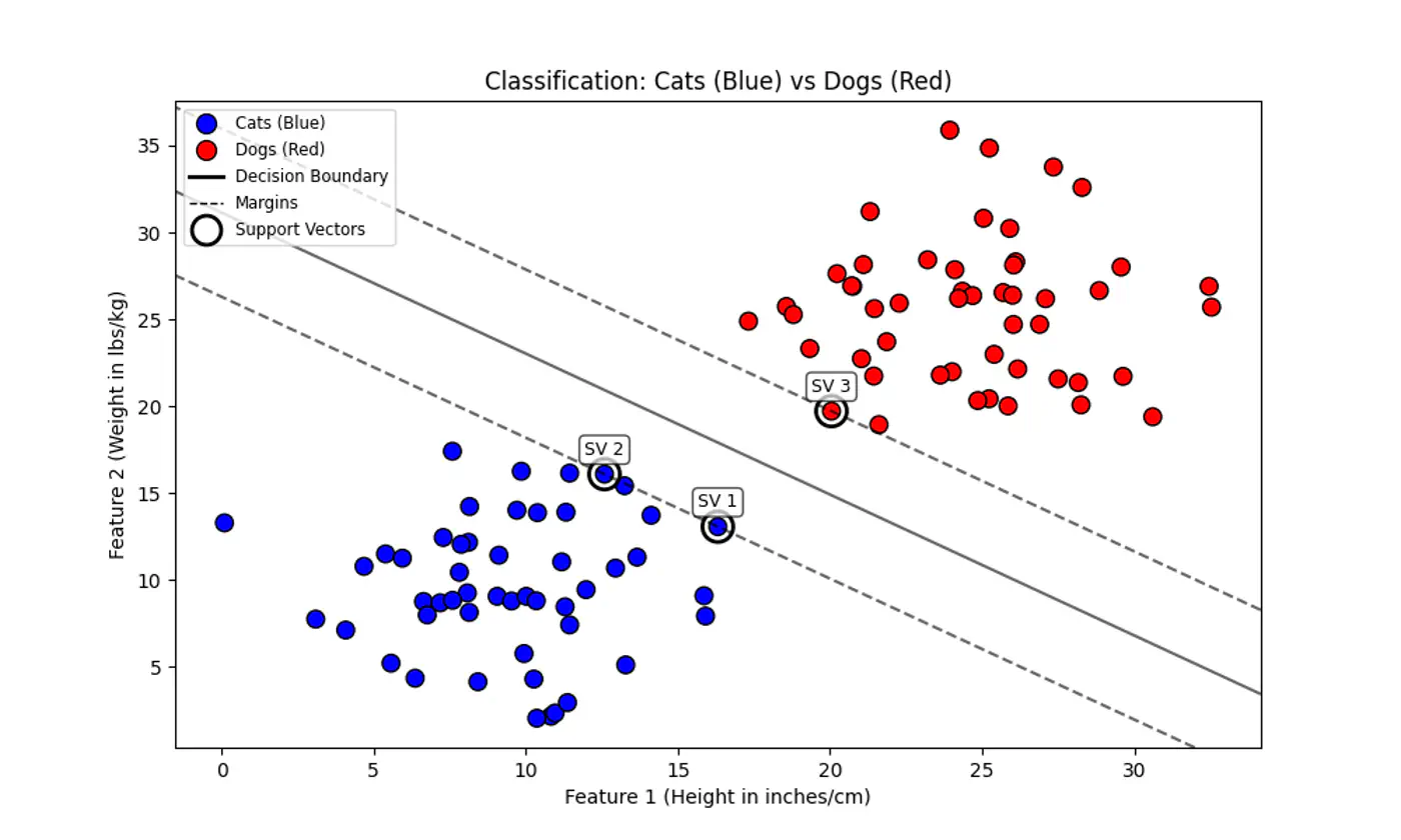
End of Section
2.5.2 - Hard Margin SVM
Data is perfectly linearly separable, i.e, there must exist a hyperplane that can perfectly separate the data into two distinct classes without any misclassification.
No noise or outliers that fall within the margin or on the wrong side of the decision boundary. Note: Even a single outlier can prevent the algorithm from finding a valid solution or drastically affect the boundary’s position, leading to poor generalization.
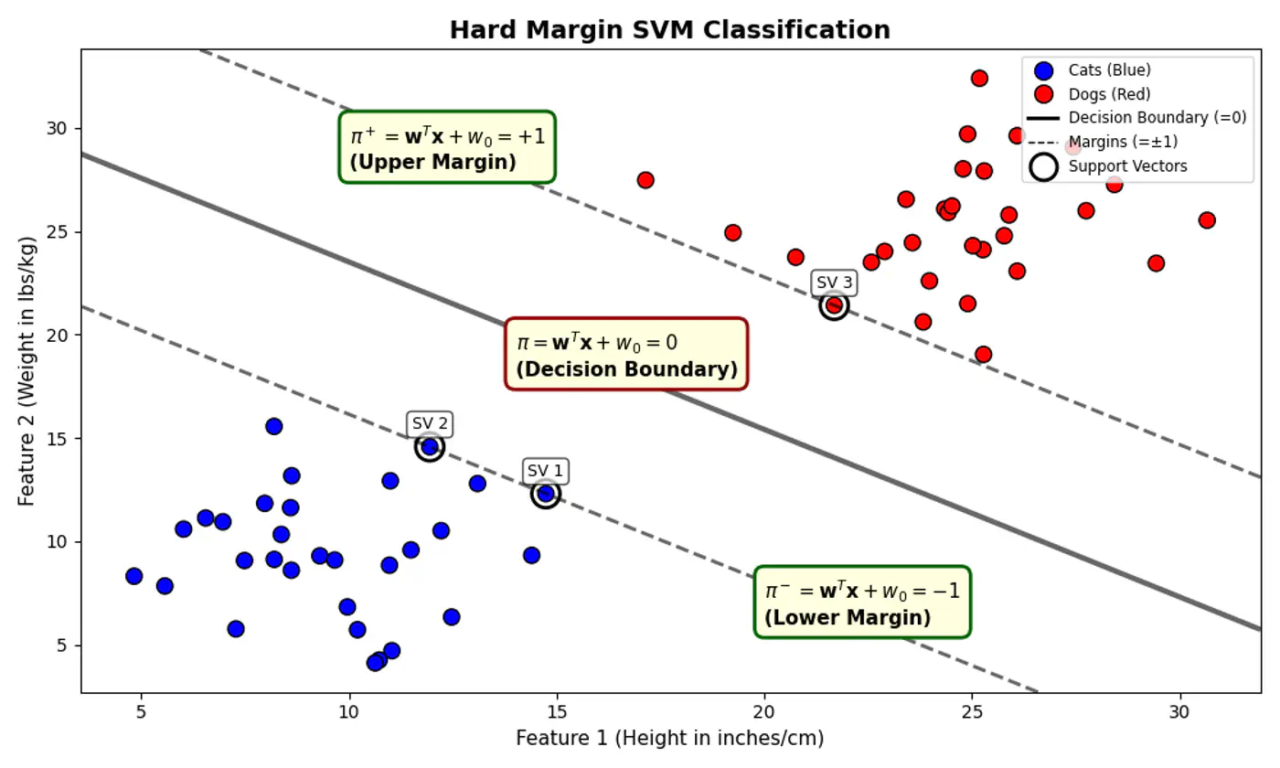
- 🐎 Distance(signed) of a hyperplane from origin = \(\frac{-w_0}{\|w\|}\)
- 🦣 Margin width = distance(\(\pi^+, \pi^-\))
- = \(\frac{1-w_0 - (-1 -w_0)}{\|w\|}\) = \(\frac{1-\cancel{w_0} + 1 + \cancel{w_0})}{\|w\|}\)
- distance(\(\pi^+, \pi^-\)) = \(\frac{2}{\|w\|}\)
Figure: Distance of Hyperplane from Origin
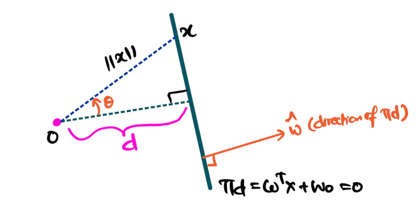
- Separating hyperplane \(\pi\) is exactly equidistant from \(\pi^+\) and \(\pi^-\).
- We want to maximize the margin between +ve(🐶) and -ve (😸) points.
👉Combining above two constraints:
\[y_{i}.(w^{T}x_{i}+w_{0})≥1\]such that, \(y_i.(w^Tx_i + w_0) \ge 1\)
👉To maximize the margin, we must minimize \(\|w\|\).
Since, distance(\(\pi^+, \pi^-\)) = \(\frac{2}{\|w\|}\)
such that, \(y_i.(w^Tx_i + w_0) \ge 1 ~ \forall i = 1,2,\dots, n\)
Note: Hard margin SVM will not work if the data has a single outlier or slight overlap.
End of Section
2.5.3 - Soft Margin SVM
💡Imagine the margin is a fence 🌉.
Hard Margin: fence is made of steel.
Nothing can cross it.Soft Margin: fence is made of rubber(porous).
Some points can ‘push’ into the margin or even cross over to the wrong side, but we charge them a penalty 💵 for doing so.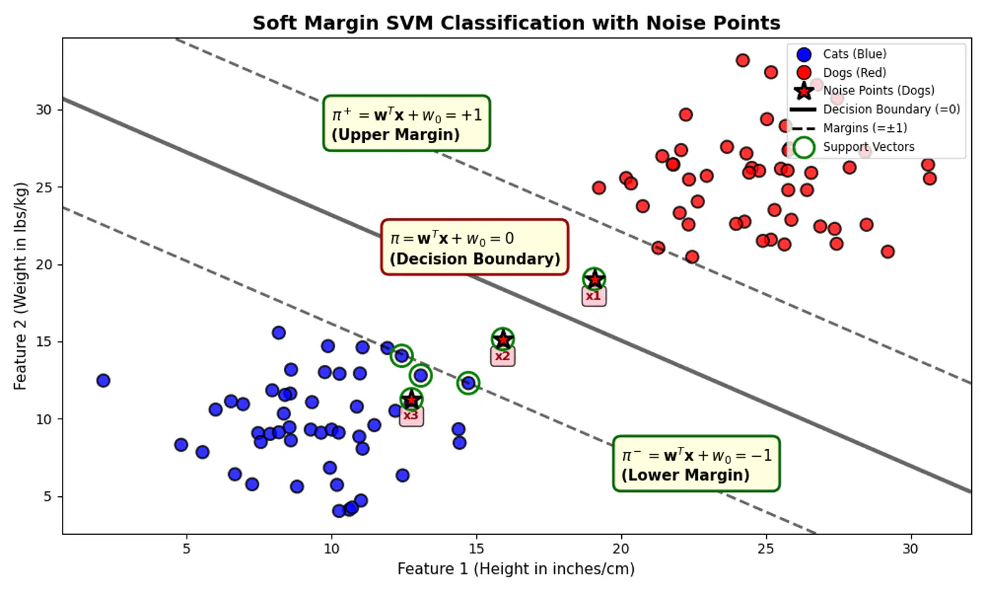
Distance from decision boundary:
- Distance of positive labelled points must be \(\ge 1\)
- But, distance of noise 📢 points (actually positive points) \(x_1, x_2 ~\&~ x_3\) < 1
⚔️ So, we introduce a slack variable or allowance for error term, \(\xi_i\) (pronounced ‘xi’) for every single data point.
\[y_i.(w^Tx_i + w_0) \ge 1 - \xi_i, ~ \forall i = 1,2,\dots, n\]\[ \implies \xi_i \ge 1 - y_i.(w^Tx_i + w_0) \\ also, ~ \xi_i \ge 0 \]\[So, ~ \xi _{i}=\max (0,1-y_{i}\cdot (w^Tx_i + w_0))\]Note: The above error term is also called ‘Hinge Loss’.
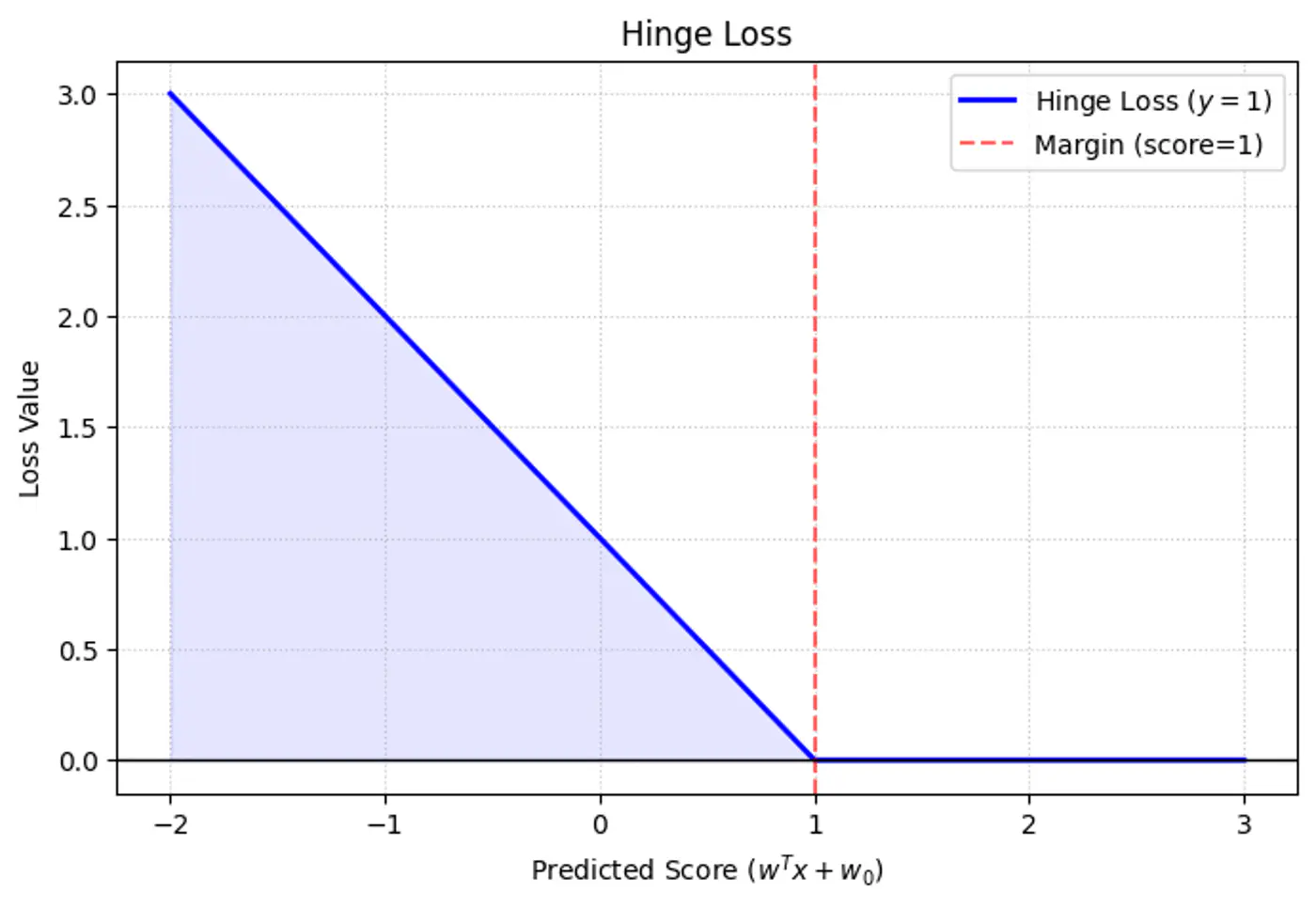
Hinge
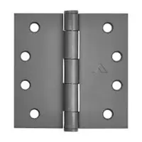
- \(\xi_i = 0\) : Correctly classified and outside (or on) the margin.
- \(0 < \xi_i \le 1 \) : Within the margin but on the correct side of the decision boundary.
- \(\xi_i > 0\): On the wrong side of the decision boundary (misclassified).
e.g.: Since, the noise 📢 point are +ve (\(y_i=1\)) labeled:
\[\xi _{i}=\max (0,1-f(x_{i}))\]\(x_1, (d=+0.5)\): \(\xi _{i}=\max (0,1-0.5) = 0.5\)
\(x_2, (d=-0.5)\): \(\xi _{i}=\max (0,1-(-0.5))= 1.5\)
\(x_3, (d=-1.5)\): \(\xi _{i}=\max (0,1-(-1.5)) = 2.5\)

Subject to constraints:
- \(y_i(w^T x_i + b) \geq 1 - \xi_i\): The ‘softened’ margin constraint.
- \(\xi_i \geq 0\): Slack/Error cannot be negative.
Note: We use a hyper-parameter ‘C’ to control the trade-off.
- Large ‘C’: Over-Fitting;
Misclassifications are expensive 💰.
Model tries to keep the errors as low as possible. - Small ‘C’: Under-Fitting;
Margin width is more important than individual errors.
Model will ignore outliers/noise to get a ‘cleaner’(wider) boundary.
Note: SVM is just L2-Regularized Hinge Loss minimization, as Logistic Regression minimizes Log-Loss.
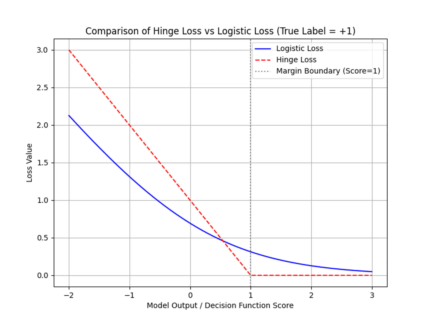
End of Section
2.5.4 - Primal Dual Equivalence
The Primal form is intuitive but computationally expensive in high dimensions.
➡️ Number of new features = \({d+p \choose p}\), grows roughly as \(O(d^{p})\)
- d= number of dimensions (features)
- p = degree of polynomial
Note: The Dual form is what enables the Kernel Trick 🪄.
Subject to constraints:
- \(y_i(w^T x_i + b) \geq 1 - \xi_i\): The ‘softened’ margin constraint.
- \(\xi_i \geq 0\): Slack/Error cannot be negative.
⭐️ We start with the Soft-Margin Primal objective and incorporate its constraints using Lagrange Multipliers \((\alpha_i, \mu_i \geq 0)\)
\[L(w, w_0, \xi, \alpha, \mu) = \frac{1}{2}\|w\|^2 + C \sum_{i=1}^n \xi_i - \sum_{i=1}^n \alpha_i \left[y_i(w^T x_i + w_0) - 1 + \xi_i \right] - \sum_{i=1}^n \mu_i \xi_i\]Note: Inequality conditions must be \(\le 0\).
👉The Lagrangian function has two competing objectives:
\[L(w, w_0, \xi, \alpha, \mu) = \frac{1}{2}\|w\|^2 + C \sum_{i=1}^n \xi_i - \sum_{i=1}^n \alpha_i \left[y_i(w^T x_i + w_0) - 1 + \xi_i \right] - \sum_{i=1}^n \mu_i \xi_i\]- Minimization: We want to minimize \(L(w, w_0, \xi, \alpha, \mu)\) w.r.t primal variables (\(w, w_0, \xi_i \) ) to find the hyperplane with the largest possible margin.
- Maximization: We want to maximize \(L(w, w_0, \xi, \alpha, \mu)\) w.r.t dual variables (\(\alpha_i, \mu_i\) ) to ensure all training constraints are satisfied.
Note: A point that is simultaneously a minimum for one set of variables and a maximum for another is, by definition, a saddle point.
👉To find the Dual, we find the saddle point by taking partial derivatives with respect to the primal variables \((w, w_0, \xi)\) and equating them to 0.
\[\frac{\partial L}{\partial w} = 0 \implies \mathbf{w = \sum_{i=1}^n \alpha_i y_i x_i}\]\[\frac{\partial L}{\partial w_0} = 0 \implies \mathbf{\sum_{i=1}^n \alpha_i y_i = 0}\]\[\frac{\partial L}{\partial \xi_i} = 0 \implies C - \alpha_i - \mu_i = 0 \implies \mathbf{0 \leq \alpha_i \leq C}\]subject to: \(0 \leq \alpha_i \leq C\) and \(\sum \alpha_i y_i = 0\)
- \(\alpha_i\)= 0, for non support vectors (correct side)
- \(0 < \alpha_i < C\), for free support vectors (exactly on the margin)
- \(\alpha_i = C\), for bounded support vectors (misclassified or inside margin)
Note: Sequential Minimal Optimization (SMO) algorithm is used to find optimal \(\alpha_i\) values.
🎯To classify unseen point \(x_q\) : \(f(x_q) = \text{sign}(w^T x_q + w_0)\)
✅ From the KKT stationarity condition, we know: \(\mathbf{w} = \sum_{i=1}^n \alpha_i y_i x_i\)
👉 Substituting this into the equation:
\[f(x_q) = \text{sign}\left( \sum_{i=1}^n \alpha_i y_i (x_i^T x_q) + w_0 \right)\]Note: Even if you have 1 million training points, if only 500 are support vectors, the summation only runs for 500 terms.
All other points have \(\alpha_i = 0\) and vanish.
End of Section
2.5.5 - Kernel Trick
👉If our data is not linearly separable in its original space , we can map it to a higher-dimensional feature space (where D»d) using a transformation function .
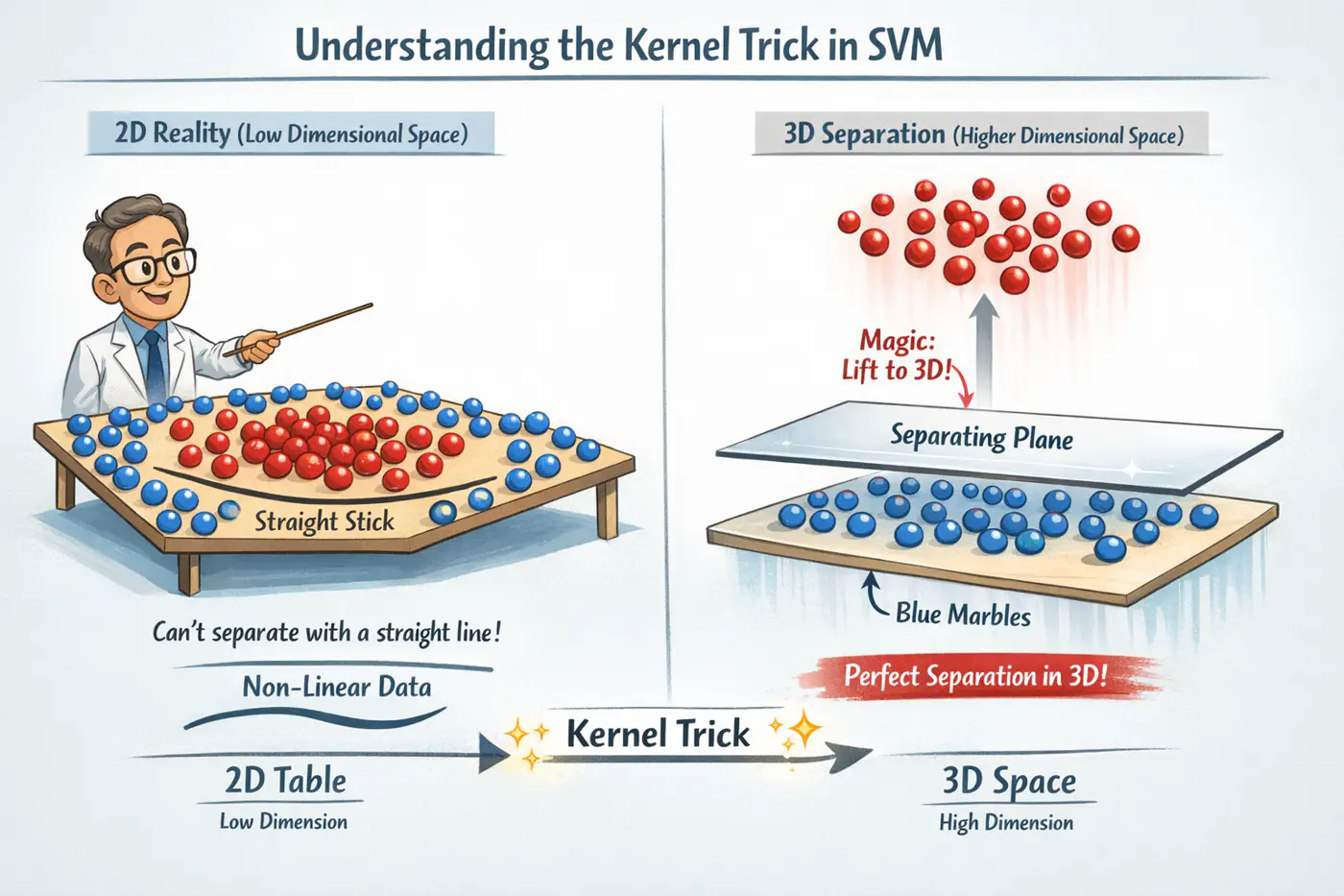
- Bridge between Dual formulation and the geometry of high dimensional spaces.
- It is a way to manipulate inner product spaces without the computational cost 💰 of explicit transformation.
subject to: \(0 \leq \alpha_i \leq C\) and \(\sum \alpha_i y_i = 0\)
💡Actual values of the input vectors \(x_i\) and \(x_j\) never appear in isolation; only appear as inner product.
\[ \max_{\alpha} \sum_{i=1}^n \alpha_i - \frac{1}{2} \sum_{i,j=1}^n \alpha_i \alpha_j y_i y_j \mathbf{(x_i \cdot x_j)}\]\[f(x_q) = \text{sign}\left( \sum_{i=1}^n \alpha_i y_i (x_i^T x_q) + w_0 \right)\]👉The ‘shape’ of the decision boundary is entirely determined by how similar points are to one another, not by their absolute coordinates.
So we define a function called ‘Kernel Function’.
The ‘Kernel Trick’ 🪄 is an optimization that replaces the dot product of a high-dimensional mapping with a function of the dot product in the original space.
\[(x_i, x_j) = \langle \phi(x_i), \phi(x_j) \rangle\]💡How it works ?
Instead of mapping (to higher dimension) \(x_i \rightarrow \phi(x_i)\), \(x_j \rightarrow \phi(x_j)\),
and calculating the dot product.
We simply compute \(K(x_i, x_j)\) directly in the original input space.
👉The ‘Kernel Function’ gives the similar mathematical equivalent of mapping it to a higher dimensions and taking the dot product.
Note: For \(K(x_i, x_j)\) to be a valid kernel, it must satisfy Mercer’s Condition.
Below is an example for a quadratic Kernel function in 2D that is equivalent to mapping the vectors to 3D and taking a dot product in 3D.
\[K(x, z) = (x^T z)^2\]\[(x_1 z_1 + x_2 z_2)^2 = x_1^2 z_1^2 + 2x_1 z_1 x_2 z_2 + x_2^2 z_2^2\]The output of above quadratic kernel function is equivalent to the explicit dot product of two vectors in 3D:
\[\phi(x) = [x_1^2, \sqrt{2}x_1x_2, x_2^2]^T\]\[\phi(z) = [z_1^2, \sqrt{2}z_1z_2, z_2^2]^T\]\[\phi (x)\cdot \phi (z)=x_{1}^{2}z_{1}^{2}+2x_{1}x_{2}z_{1}z_{2}+x_{2}^{2}z_{2}^{2}\]- Computational Efficiency: Avoids the ‘combinatorial blowup’ 💥 of generating thousands of interaction features manually.
- Memory Savings: No need to store 💾 or process high-dimensional coordinates, only the scalar result of the kernel function.
- Designing special purpose domain specific kernel is very hard.
- Basically, we are trying to replace feature engineering with kernel design.
- Note: Deep learning does feature engineering implicitly for us.
- Runtime complexity depends on number of support vectors, whose count is not easy to control.
Note: Runtime Time Complexity ⏰ = \(O(n_{SV}\times d)\) , whereas linear SVM,\(O(d)\) .
End of Section
2.5.6 - RBF Kernel
- Unlike the polynomial kernel, which looks at global 🌎 interactions, the RBF kernel acts like a similarity measure.
- If ‘x’ and ‘z’ are identical \(K(x,z)=1\).
- As they move further apart in Euclidean space, the value decays exponentially towards 0.
- If \(x \approx z\) (very close), \(K(x,z)=1\)
- If ‘x’, ‘z’ are far apart, \(K(x,z) \approx 0\)
Note: Kernel function is the measure of similarity or closeness.
Say \(\sigma = 1\), then Euclidean distance: \(\|x - z\|^2 = \|x\|^2 + \|z\|^2 - 2x^Tz\)
\[K(x, z) = \exp(-( \|x\|^2 + \|z\|^2 - 2x^T z )) = \exp(-\|x\|^2) \exp(-\|z\|^2) \exp(2x^T z)\]The Taylor expansion for \(e^u= \sum_{n=0}^{\infty} \frac{u^n}{n!}\)
\[\exp(2x^T z) = \sum_{n=0}^{\infty} \frac{(2x^T z)^n}{n!} = 1 + \frac{2x^T z}{1!} + \frac{(2x^T z)^2}{2!} + \dots + \frac{(2x^T z)^n}{n!} + \dots\]\[K(x, z) = e^{-\|x\|^2} e^{-\|z\|^2} \left( \sum_{n=0}^{\infty} \frac{2^n (x^T z)^n}{n!} \right)\]💡If we expand each \((x^T z)^n\) term, it represents the dot product of all possible n-th order polynomial features.
👉Thus, the implicit feature map is:
\[\phi(x) = e^{-\|x\|^2} \left[ 1, \sqrt{\frac{2}{1!}}x, \sqrt{\frac{2^2}{2!}}(x \otimes x), \dots, \sqrt{\frac{2^n}{n!}}(\underbrace{x \otimes \dots \otimes x}_{n \text{ times}}), \dots \right]^T\]- Important: The tensor product \(x\otimes x\) creates a vector (or matrix) containing all combinations of the features. e.g. if \(x=[x_{1},x_{2}]\), then \(x\otimes x=[x_{1}^{2},x_{1}x_{2},x_{2}x_{1},x_{2}^{2}]\) 
Note: Because the Taylor series has an infinite number of terms, feature map has an infinite number of dimensions.
- High Gamma(low \(\sigma\)): Over-Fitting
- Makes the kernel so ‘peaky’ that each support vector only influences its immediate neighborhood.
- Decision boundary becomes highly irregular, ‘wrapping’ tightly around individual data points to ensure they are classified correctly.
- Low Gamma(high \(\sigma\)): Under-Fitting
- The Gaussian bumps are wide and flat.
- Decision boundary becomes very smooth, essentially behaving more like a linear or low-degree polynomial classifier.
End of Section
2.5.7 - Support Vector Regression
👉Imagine a ‘tube’ of radius \(\epsilon\) surrounding the regression line.
- Points inside the tube are considered ‘correct’ and incur zero penalty.
- Points outside the tube are penalized based on their distance from the tube’s boundary.
👉SVR ignores errors as long as they are within a certain distance (\(\epsilon\)) from the true value.
🎯This makes SVR inherently robust to noise and outliers, as it does not try to fit every single point perfectly, only those that ‘matter’ to the structure of the data.
Note: Standard regression (like OLS) tries to minimize the squared error between the prediction and every data point.
Subject to constraints:
- \(y_i - (w^T x_i + w_0) \leq \epsilon + \xi_i\): (Upper boundary)
- \((w^T x_i + w_0) - y_i \leq \epsilon + \xi_i^*\): (Lower boundary)
- \(\xi_i, \xi_i^* \geq 0\): (Slack/Error cannot be negative)
Terms:
- Epsilon(\(\epsilon\)): The width of the tube. Increasing ‘\(\epsilon\)’ results in fewer support vectors and a smoother (flatter) model.
- Slack Variables (\(\xi_i, \xi_i^*\)): How far a point lies outside the upper and lower boundaries of the tube.
- C: The trade-off between the flatness of the model and the extent to which deviations larger than \(\epsilon\) are tolerated.
SVR uses a specific loss function that is 0 when the error<’\(\epsilon\)’.
\[L_\epsilon(y, f(x)) = \max(0, |y - f(x)| - \epsilon)\]- The solution becomes sparse, because the loss is zero for points inside the tube.
- Only the Support Vectors, i.e, points outside or on the boundary of the tube have non-zero Lagrange multipliers (\(\alpha_i\)).
Note: \(\epsilon=0.1\) default value in scikit-learn.
Subject to:
- \(\sum_{i=1}^n (\alpha_i - \alpha_i^*) = 0\)
- \(0 \leq \alpha_i, \alpha_i^* \leq C\)
- \(\alpha_i = \alpha_i^* = 0\): point is inside the tube.
- \(|\alpha_i - \alpha_i^*| > 0\) : support vectors; points on or outside the tube.
Note: \(\alpha_i , \alpha_i^* \) cannot both be non-zero for the same point; a point cannot be simultaneously above and below the tube.
- 👉 For non-linear SVR we replace dot product \(x_i^T x_j\) with kernel function \(K(x_i, x_j)\).
- ✅ Model needs to store only support vectors, i.e, points where \(|\alpha_i - \alpha_i^*| > 0\).
- ⭐️\(\xi_i =0 \) for a point that lies exactly on the boundary, so we can use that to calculate the bias (\(w_0\)):
End of Section
2.6.1 - Naive Bayes Intro
📌 Let’s understand Naive Bayes through an Email/Text classification example.
- Number of words in an email is not fixed.
- Remove all stop words, such as, the, is , are, if, etc.
- Keep only relevant words, i.e, \(w_1, w_2, \dots , w_d\) words.
- We want to do a binary classification - Spam/Not Spam.
Let’s revise Bayes’ theorem first:
- \(P(S|W)\) is the posterior probability: the probability of the email being spam, given the words inside it.
- \(P(W|S)\) is the likelihood: how likely is this email’s word pattern if it were spam?
- \(P(S)\) is the prior probability: The ‘base rate’ of spam.
- If our dataset has 10,000 emails and 2,000 are spam, then \(P(S)\)=0.2.
- \(P(W)\) is the prior probability of the predictor (evidence): total probability of seeing these words across all emails.
- 👉Since this is the same for both classes, we treat it as a constant and ignore it during comparison.
👉 Likelihood = \(P(W|S)\) = \(P(w_1, w_2, \dots w_d | S)\)
➡️ For computing the joint distribution of say d=1000 words, we need to learn from possible \(2^{1000}\) combinations.
- \(2^{1000}\) > the atoms in the observable 🔭 universe 🌌.
- We will never have enough training data to see every possible combination of words even once.
- Most combinations would have a count of zero.
🦉 So, how do we solve this ?
💡 The ‘Naive’ assumption is a ‘Conditional Independence’ assumption, i.e, we assume each word appears independently of the others, given the class Spam/Not Spam.
- e.g. In a spam email, the likelihood of ‘Free’ and ‘Money’ 💵 appearing are treated as independent events, even though they usually appear together.
Note: The conditional independence assumption makes the probability calculations easier, i.e, the joint probability simply becomes the product of individual probabilities, conditional on the label.
\[P(W|S) = P(w_1|S)\times P(w_2|S)\times \dots P(w_d|S) \]\[\implies P(S|W)=\frac{P(w_1|S)\times P(w_2|S)\times \dots P(w_d|S)\times P(S)}{P(W)}\]\[\implies P(S|W)=\frac{\prod_{i=1}^d P(w_i|S)\times P(S)}{P(W)}\]\[\text{Similarly, } P(NS|W)=\frac{\prod_{i=1}^d P(w_i|NS)\times P(NS)}{P(W)}\]We can generalize it for any number of class labels ‘y’:
Note: We compute the probabilities for both Spam/Not Spam and assign the final label to email, depending upon which probability is higher.
👉 Space Complexity: O(d*c)
👉 Time Complexity:
- Training: O(n*d*c)
- Inference: O(d*c)
Where,
- d = number of features/dimensions
- c = number of classes
- n = number of training examples
End of Section
2.6.2 - Naive Bayes Issues
⭐️ Simple, fast, and highly effective probabilistic machine learning classifier based on Bayes’ theorem.
\[P(y|W) \propto \prod_{i=1}^d P(w_i|y)\times P(y)\]\[P(w_i|y) = \frac{count(w_i ~in~ y)}{\text{total words in class y}}\]🦀 What if at runtime we encounter a word that was never seen during training ?
e.g. A word ‘crypto’ appears in the test email that was not present in training emails; P(‘crypto’|S) =0.
👉 This will force the entire product to zero.
\[P(w_i|S) = \frac{\text{Total count of } w_i \text{ in all Spam emails}}{\text{Total count of all words in all Spam emails}}\]💡 Add ‘Laplace smoothing’ to all likelihoods, both during training and test time, so that the probability becomes non-zero.
\[P(x_{i}|y)=\frac{count(x_{i},y)+\alpha }{count(y)+\alpha \cdot |V|}\]- \(count(x_{i},y)\) : number of times word appears in documents of class ‘y'.
- \(count(y)\): The total count of all words in documents of class ‘y'.
- \(|V|\)(or \(N_{features}\)):Vocabulary size or total number of unique possible words.
Let’s understand this by the examples below:
\[P(w_{i}|S)=\frac{count(w_{i},S)+\alpha }{count(S)+\alpha \cdot |V|}\]- \(count(w_{i},S) = 0 \), \(count(S) = 100\), \(|V|\)(or \(N_{features}) =2, \alpha = 1\) \[P(w_{i}|S)=\frac{ 0+1 }{100 +1 \cdot 2} = \frac{1}{102}\]
- \(count(w_{i},S) = 0 \), \(count(S) = 100\), \(|V|\)(or \(N_{features}) =2, \alpha = 10,000\) \[P(w_{i}|S)=\frac{ 0+10,000 }{100 +10,000 \cdot 2} = \frac{10,000}{20,100} \approx \frac{1}{2}\]
Note: High alpha value may lead to under-fitting; \(\alpha = 1\) recommended.
🦀 What happens if the number of words ‘d’ is very large ?
👉 Multiplying 500 times will result in a number so small a computer 💻 cannot store it (underflow).
Note: Computers have a limit to store floating point numbers, e.g., 32 bit: \(1.175 x 10^{-38}\)
💡 Take ‘Logarithm’ that will convert the product to sum.
\[P(y|W) \propto \prod_{i=1}^d P(w_i|y)\times P(y)\]\[\log(P(y| W)) \propto \sum_{i=1}^d \log(P(w_i|y)) + \log(P(y))\]Note: In the next section we will solve a problem covering all the concepts discussed in this section.
End of Section
2.6.3 - Naive Bayes Example
⭐️ Simple, fast, and highly effective probabilistic machine learning classifier based on Bayes’ theorem.
\[\log(P(y| W)) \propto \sum_{i=1}^d \log(P(w_i|y)) + \log(P(y))\]\[P(w_{i}|y)=\frac{count(w_{i},y)+\alpha }{count(y)+\alpha \cdot |V|}\]Let’s solve an email classification problem, below we have list of emails (tokenized) and labelled as Spam/Not Spam for training.
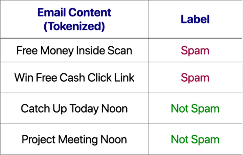
🏛️ Class Priors:
- P(Spam) = 2/4 =0.5
- P(Not Spam) = 2/4 = 0.5
📕 Vocabulary = { Free, Money, Inside, Scan, Win, Cash, Click, Link, Catch, Up Today, Noon, Project, Meeting }
- |V| = Total unique word count = 14
🧮 Class count:
- count(Spam) = 9
- count(Not Spam) = 7
✅ Laplace smoothing: \(\alpha = 1\)
- P(‘free’| Spam) = \(\frac{2+1}{9+14} = \frac{3}{23} = 0.13\)
- P(‘free’| Not Spam) = \(\frac{0+1}{7+14} = \frac{1}{21} = 0.047\)
👉 Say a new email 📧 arrives - “Free money today”; lets classify it as Spam/Not Spam.
Spam:
- P(‘free’| Spam) = \(\frac{2+1}{9+14} = \frac{3}{23} = 0.13\)
- P(‘money’| Spam) = \(\frac{1+1}{9+14} = \frac{2}{23} = 0.087\)
- P(‘today’| Spam) = \(\frac{0+1}{9+14} = \frac{1}{23} = 0.043\)
Not Spam:
- P(‘free’| Not Spam) = \(\frac{0+1}{7+14} = \frac{1}{21} = 0.047\)
- P(‘money’| Not Spam) = \(\frac{0+1}{7+14} = \frac{1}{21} = 0.047\)
- P(‘today’| Not Spam) = \(\frac{1+1}{7+14} = \frac{2}{21} = 0.095\)
- Score(Spam) = log(P(Spam)) + log(P(‘free’|S)) + log(P(‘money’|S)) + log(P(‘today’|S))
= log(0.5) + log(0.13) + log(0.087) + log(0.043) = -0.301 -0.886 -1.06 -1.366 = -3.614 - Score(Not Spam) = log(P(Not Spam)) + log(P(‘free’|NS)) + log(P(‘money’|NS)) + log(P(‘today’|NS))
= log(0.5) + log(0.047) + log(0.047) + log(0.095) = -0.301 -1.328 -1.328 -1.022 = -3.979
👉 Since, Score(Spam) (-3.614 )> Score(Not Spam) (-3.979) , the model chooses ‘Spam’ as the label for the email.
End of Section
3 - Unsupervised Learning
3.1.1 - K Means
🌍In real-world systems, labeled data is scarce and expensive 💰.
💡Unsupervised learning discovers inherent structure without human annotation.
👉Clustering answers: “Given a set of points, what natural groupings exist?”
- Customer Segmentation: Group users by behavior without predefined categories.
- Image Compression: Reduce color palette by clustering pixel colors.
- Anomaly Detection: Points far from any cluster are outliers.
- Data Exploration: Understand structure before building supervised models.
- Preprocessing: Create features from cluster assignments.
💡Clustering assumes that ‘similar’ points should be grouped together.
👉But what is ‘similar’? This assumption drives everything.
Given:
- Dataset X = {x₁, x₂, …, xₙ} where xᵢ ∈ ℝᵈ.
- Desired number of clusters ‘k'.
Find:
Cluster assignments C = {C₁, C₂, …, Cₖ}.
Such that points within clusters are ‘similar’.
And points across clusters are ‘dissimilar’.
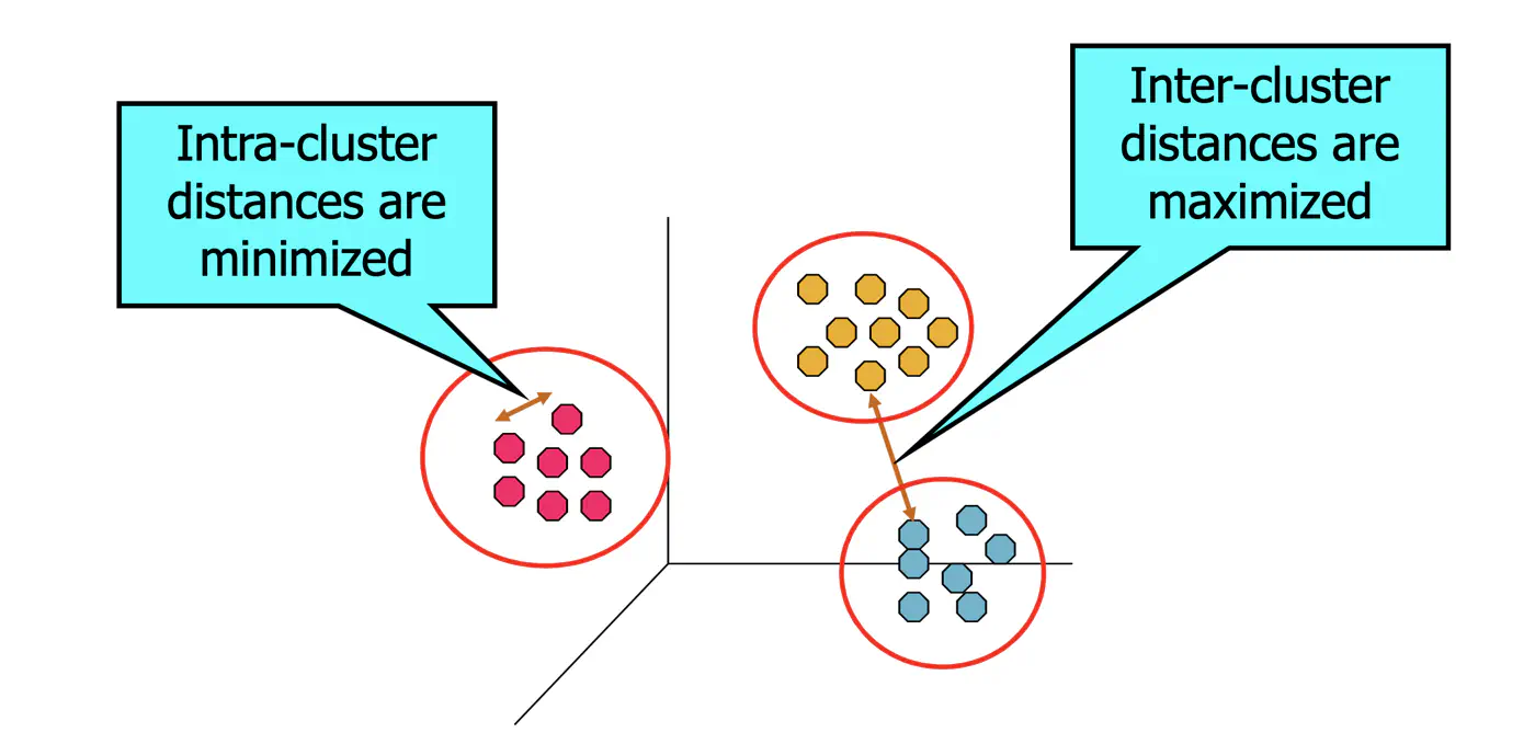
This is fundamentally an optimization problem, i.e, find parameters such that the value is minimum/maximum. We need:
- An objective function
- what makes a clustering ‘good’?
- An algorithm to optimize it
- how do we find good clusters?
- Evaluation metrics
- how do we measure quality?
Objective function:
👉Minimize the within-cluster sum of squares (WCSS).
- Where:
- C = {C₁, …, Cₖ} are cluster assignments.
- μⱼ is the centroid (mean) of cluster Cₖ.
- ||·||² is squared Euclidean distance.
Note: Every point belongs to one and only one cluster.
💡Within-Cluster Sum of Squares (WCSS) is nothing but variance.
⭐️ Total Variance = Within-Cluster Variance + Between-Cluster Variance
👉K-Means minimizes within-Cluster variance, which implicitly maximizes between-cluster separation.
Geometric Interpretation:
- Each point is ‘pulled’ toward its cluster center.
- The objective measures total squared distance of all points to their centers.
- Lower J(C, μ) means tighter, more compact clusters.
Note: K-Means works best when clusters are roughly spherical, similarly sized, and well-separated.
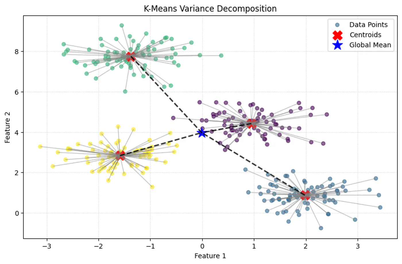
⭐️The problem requires partitioning ’n’ observations into ‘k’ distinct, non-overlapping clusters, which is given by the Stirling number of the second kind, which grows at a rate roughly equal to \(k^n/k!\).
\[S(n,k)=\frac{1}{k!}\sum _{j=0}^{k}(-1)^{k-j}{k \choose j}j^{n}\]\[S(100,2)=2^{100-1}-1=2^{99}-1\]\[2^{99}\approx 6.338\times 10^{29}\]👉This large number of possible combinations makes the problem NP-Hard.
🦉The k-means optimization problem is NP-hard because it belongs to a class of problems for which no efficient (polynomial-time ⏰) algorithm is known to exist.
End of Section
3.1.2 - Lloyds Algorithm
Iterative method for partitioning ’n’ data points into ‘k’ groups by repeatedly assigning data points to the nearest centroid (mean) and then recalculating centroids until assignments stabilize, aiming to minimize within-cluster variance.
📥Input: X = {x₁, …, xₙ}, ‘k’ (number of clusters)
📤Output: ‘C’ (clusters), ‘μ’ (centroids)
👉Steps:
- Initialize: Randomly choose ‘k’ cluster centroids μ₁, …, μₖ.
- Repeat until convergence, i.e, until cluster assignments and centroids no longer change significantly.
- a) Assignment: Assign each data point to the cluster whose centroid is closest (usually using Euclidean distance).
- For each point xᵢ: cᵢ = argminⱼ ||xᵢ - μⱼ||²
- b) Update: Recalculate the centroid (mean) of each cluster.
- For each cluster j: μⱼ = (1/|Cⱼ|) Σₓᵢ∈Cⱼ xᵢ
- Initialization sensitive, different initialization may lead to different clusters.
- Tries to make each cluster of same size that may not be the case in real world.
- Tries to make each cluster with same density(variance)
- Does not work well with non-globular(spherical) data.
👉See how 2 different runs of K-Means algorithm gives totally different clusters.

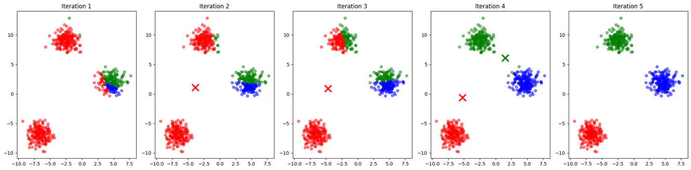
👉Also, K-Means does not work well with non-spherical clusters, or clusters with different densities and sizes.
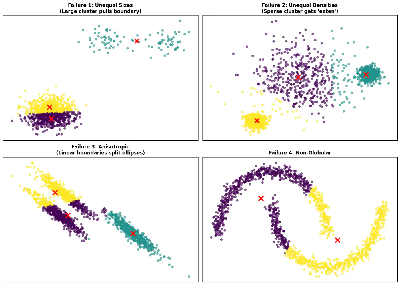
✅ Do not select initial points randomly, but some logic, such as, K-means++ algorithm.
✅ Use hierarchical clustering or density based clustering DBSCAN.
End of Section
3.1.3 - K Means++
- If two initial centroids belong to the same natural cluster, the algorithm will likely split that natural cluster in half and be forced to merge two other distinct clusters elsewhere to compensate.
- Inconsistent; different runs may lead to different clusters.
- Slow convergence; Centroids may need to travel much farther across the feature space, requiring more iterations.
👉Example for different K-Means algorithm runs give different clusters
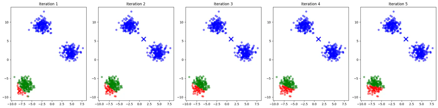

💡Addresses the issue due to random initialization by aiming to spread out the initial centroids across the data points.
Steps:
- Select the first centroid: Choose one data point randomly from the dataset to be the first centroid.
- Calculate distances: For every data point x not yet selected as a centroid, calculate the distance, D(x), between x and the nearest centroid chosen so far.
- Select the next centroid: Choose the next centroid from the remaining data points with a probability
proportional to D(x)^2.
This makes it more likely that a point far from existing centroids is selected, ensuring the initial centroids are well-dispersed. - Repeat: Repeat steps 2 and 3 until ‘k’ number of centroids are selected.
- Run standard K-means: Once the initial centroids are chosen, the standard k-means algorithm proceeds with assigning data points to the nearest centroid and iteratively updating the centroids until convergence.
End of Section
3.1.4 - K Medoid
- In K-Means, the centroid is the arithmetic mean of the cluster. The mean is very sensitive to outliers.
- Not interpretable; centroid is the mean of cluster data points and may not be an actual data point, hence not representative.
⭐️Medoid is a specific data point from a dataset that acts as the ‘center’ or most representative member of its cluster.
👉It is defined as the object within a cluster whose average dissimilarity (distance) to all other members in that same cluster is the smallest.
💡Selects actual data points from the dataset as cluster representatives, called medoids (most centrally located).
👉a.k.a Partitioning Around Medoids(PAM).
Steps:
- Initialization: Select ‘k’ data points from the dataset as the initial medoids using K-Means++ algorithm.
- Assignment: Calculate the distance (e.g., Euclidean or Manhattan) from each non-medoid point to all medoids and assign each point to the cluster of its nearest medoid.
- Update (Swap):
- For each cluster, swap current medoid with a non-medoid point from the same cluster.
- For each swap, calculate the total cost 💰(sum of distances from medoid).
- Pick the medoid with minimum cost 💰.
- Repeat🔁: Repeat the assignment and update steps until (convergence), i.e, medoids no longer change or a maximum number of iterations is reached.
Note: Kind of brute-force algorithm, computationally expensive for large dataset.
✅ Flexible Distance Metrics: It can work with any dissimilarity measure (Manhattan, Cosine similarity), making it ideal for categorical or non-Euclidean data.
✅ Interpretable Results: Cluster centers are real observations (e.g., a ‘typical’ customer profile), which makes the output easier to explain to stakeholders.
End of Section
3.1.5 - Clustering Quality Metrics
- 👉 Elbow Method: Quickest to compute; good for initial EDA (Exploratory Data Analysis).
- 👉 Dunn Index: Focuses on the ‘gap’ between the closest clusters.
- 👉 Silhouette Score: Balances compactness and separation.
- 👉 Domain specific knowledge and system constraints.
⭐️Heuristic used to determine the optimal number of clusters (k) for clustering by visualizing how the quality of clustering improves as ‘k’ increases.
🎯The goal is to find a value of ‘k’ where adding more clusters provides a diminishing return in terms of variance reduction.
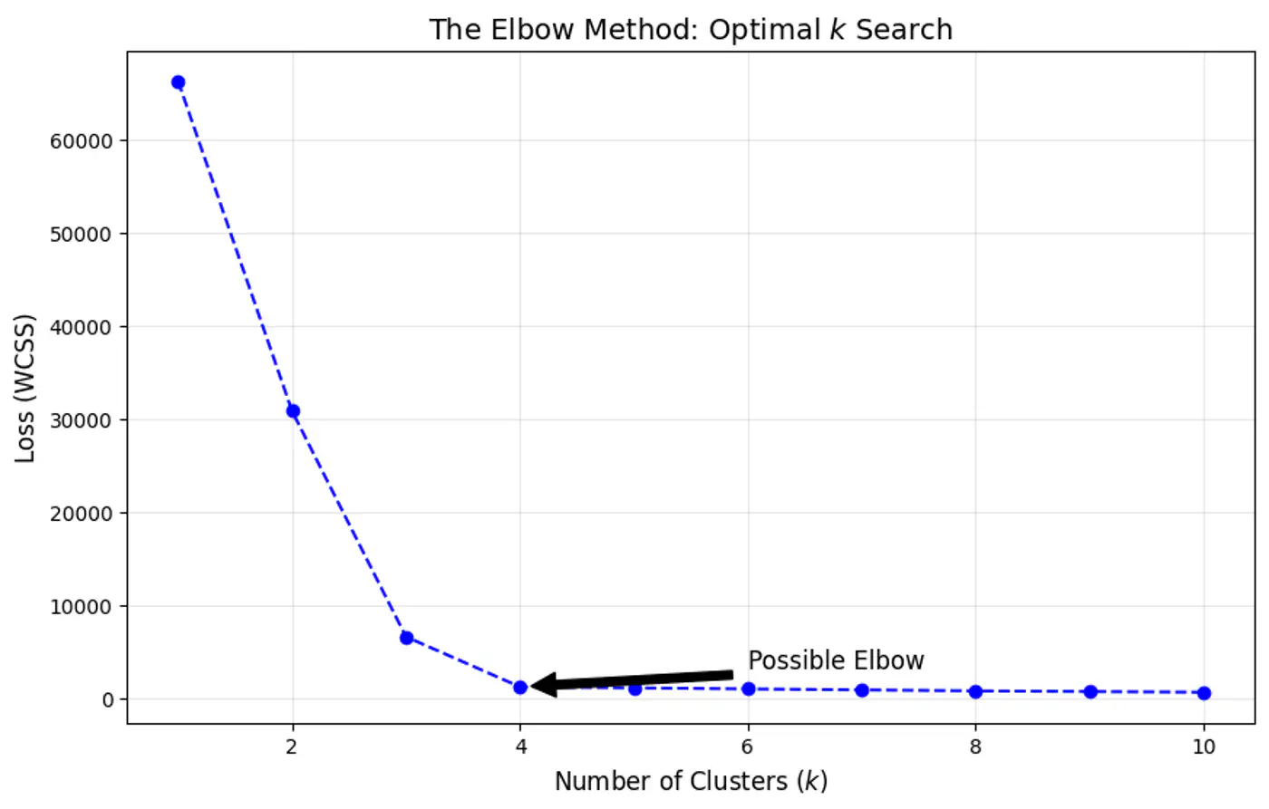
⭐️Clustering quality evaluation metric that measures: separation (between clusters) and compactness (within clusters)
Note: A higher Dunn Index value indicates better clustering, meaning clusters are well-separated from each other and compact.
👉Dunn Index Formula:
\[DI = \frac{\text{Minimum Inter-Cluster Distance(between different clusters)}}{\text{Maximum Intra-Cluster Distance(within a cluster)}}\]\[DI = \frac{\min_{1 \le i < j \le k} \delta(C_i, C_j)}{\max_{1 \le l \le k} \Delta(C_l)}\]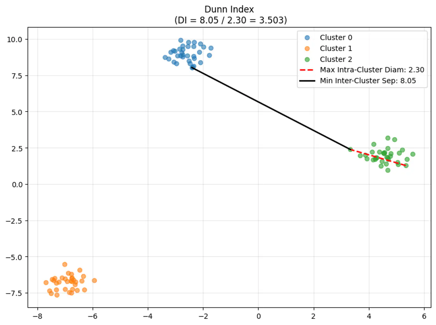
👉Let’s understand the terms in the above formula:
\(\delta(C_i, C_j)\) (Inter-Cluster Distance):
- Measures how ‘far apart’ the clusters are.
- Distance between the two closest points of different clusters (Single-Linkage distance). \[\delta(C_i, C_j) = \min_{x \in C_i, y \in C_j} d(x, y)\]
\(\Delta(C_l)\) (Intra-Cluster Diameter):
- Measures how ‘spread out’ a cluster is.
- Distance between the two furthest points within the same cluster (Complete-Linkage distance). \[\Delta(C_l) = \max_{x, y \in C_l} d(x, y)\]
- Single Linkage (MIN): Uses the minimum distance between any two points in different clusters.
- Complete Linkage (MAX): Uses the maximum distance between any two points in same cluster.
End of Section
3.1.6 - Silhouette Score
- ✅ Elbow Method: Quickest to compute; good for initial EDA.
- ✅ Dunn Index: Focuses on the ‘gap’ between the closest clusters.
——- We have seen the above 2 methods in the previous section ———- - 👉 Silhouette Score: Balances compactness and separation.
- 👉 Domain specific knowledge and system constraints.
⭐️Clustering quality evaluation metric that measures how similar a data point is to its own cluster (cohesion) compared to other clusters (separation).
Note: Higher scores (closer to 1) indicate better-defined, distinct clusters, while scores near 0 suggest overlapping clusters, and negative scores mean points might be in the wrong cluster.
Silhouette score for point ‘i’ is the difference between separation b(i) and cohesion a(i), normalized by the larger of the two.
\[ s(i) = \frac{b(i) - a(i)}{\max(a(i), b(i))} \]Note: The Global Silhouette Score is simply the mean of s(i) for all points in the dataset.
👉Example for Silhouette Score:
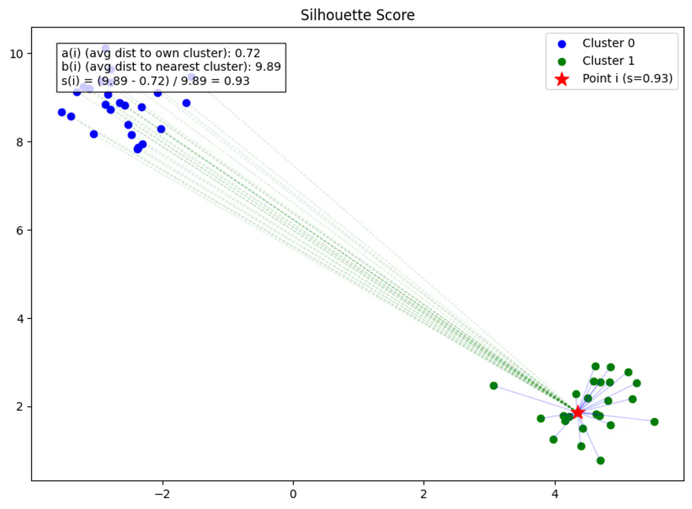
👉Example for Silhouette Score of 0(Border Point) and negative(Wrong Cluster).
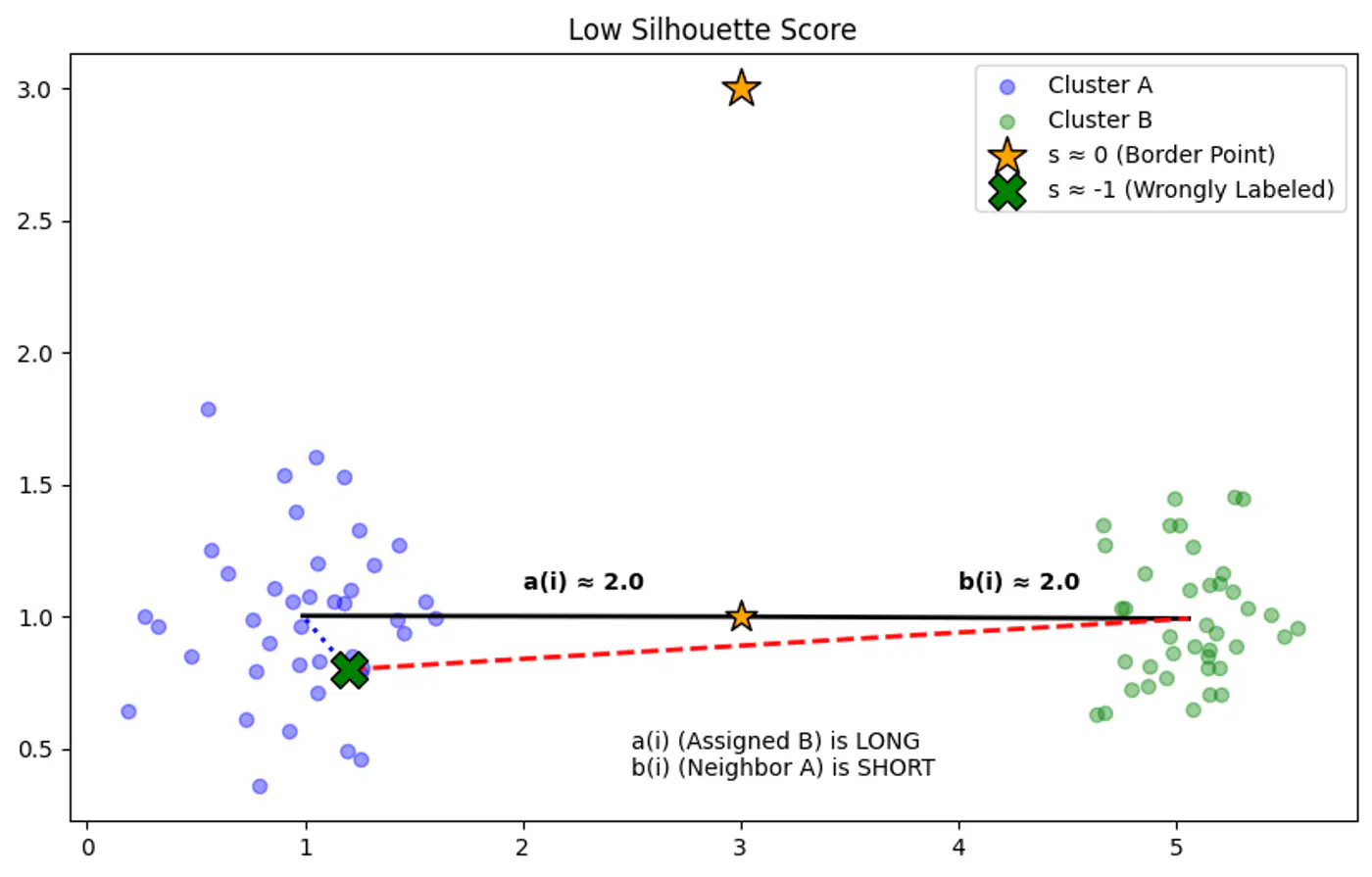
🦉Now let’s understand the terms in Silhouette Score in detail.
Average distance between point ‘i’ and all other points in the same cluster.
\[a(i) = \frac{1}{|C_A| - 1} \sum_{j \in C_A, i \neq j} d(i, j)\]Note: Lower a(i) means the point is well-matched to its own cluster.
Average distance between point ‘i’ and all points in the nearest neighboring cluster (the cluster that ‘i’ is not a part of, but is closest to).
\[b(i) = \min_{C_B \neq C_A} \frac{1}{|C_B|} \sum_{j \in C_B} d(i, j)\]Note: Higher b(i) means the point is very far from the next closest cluster.
⭐️A silhouette plot is a graphical tool used to evaluate the quality of clustering algorithms (like K-Means), showing how well each data point fits within its cluster.
👉Each bar gives the average silhouette score of the points assigned to that cluster.
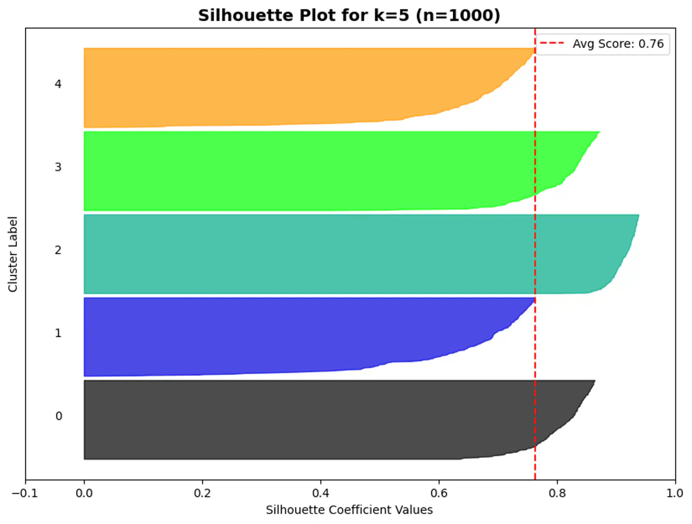
⛳️ Like K-Means, the Silhouette Score (when using Euclidean distance) assumes convex clusters.
🌘 If we use it on ‘Moon’ shaped clusters, it will give a low score even if the clusters are perfectly separated, because the ‘average distance’ to a neighbor might be small due to the curvature of the manifold.
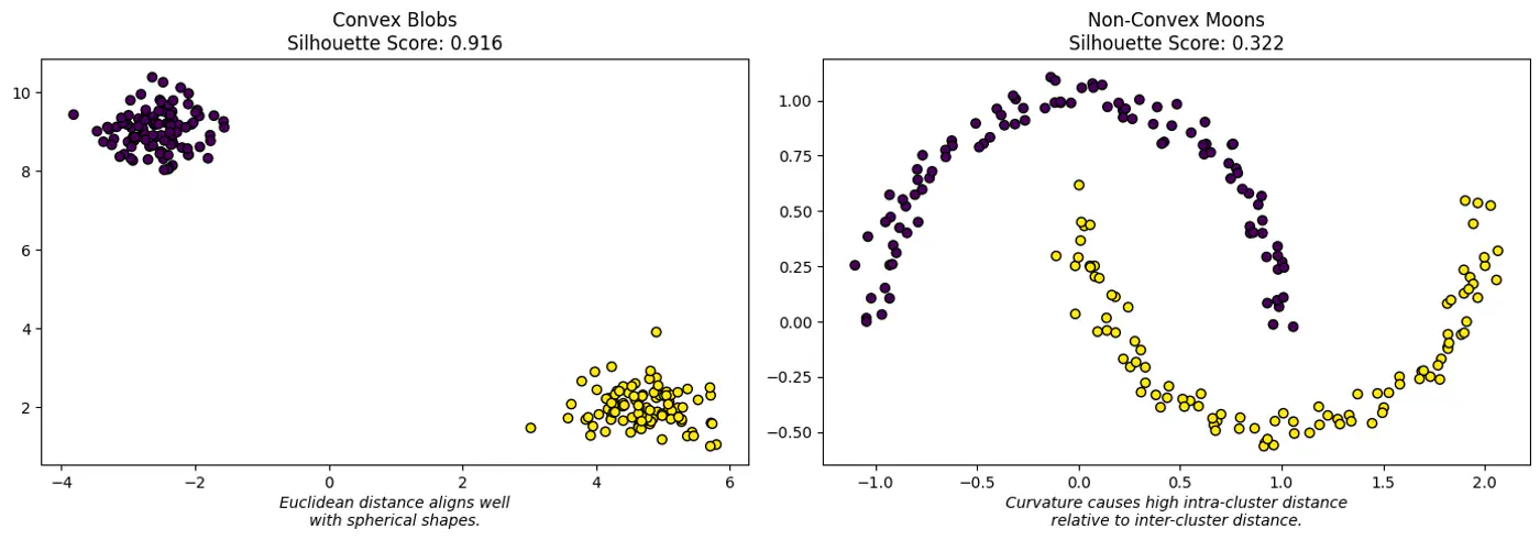
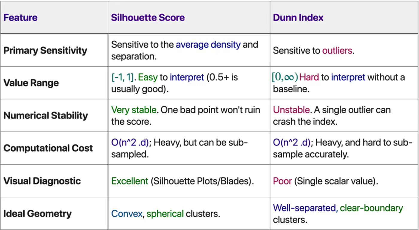
Choose Silhouette Score if:
✅ Need a human-interpretable metric to present to stakeholders.
✅ Dealing with real-world noise and overlapping ‘fuzzy’ boundaries.
✅ Want to see which specific clusters are weak (using the plot).
Choose Dunn Index if:
✅ Performing ‘Hard Clustering’ where separation is a safety or business requirement.
✅ Data is pre-cleaned of outliers (e.g., in a curated embedding space).
✅ Need to compare different clustering algorithms (e.g., K-Means vs. DBSCAN) on a high-integrity task.
End of Section
3.2 - Hierarchical Clustering
3.2.1 - Hierarchical Clustering
- 🤷 We might not know in advance the number of distinct clusters ‘k’ in the dataset.
- 🕸️ Also, sometimes the dataset may contain a nested structure or some inherent hierarchy, such as, file system, organizational chart, biological lineages, etc.
⭐️ Method of cluster analysis that seeks to build a hierarchy of clusters, resulting in a tree like structure called dendrogram.
👉Hierarchical clustering allows us to explore different possibilities (of ‘k’) by cutting the dendrogram at various levels.
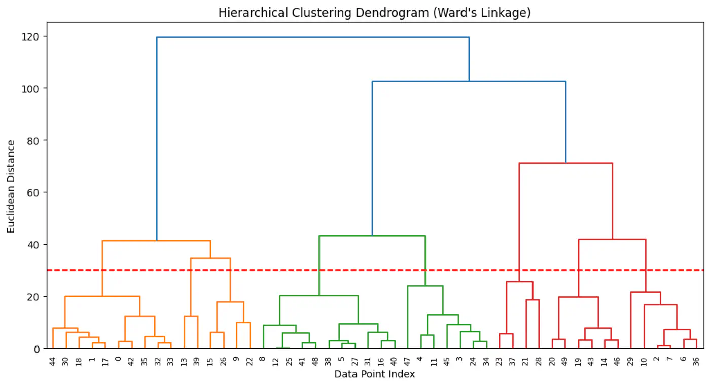
Agglomerative (Bottom-Up):
Most common, also known as Agglomerative Nesting (AgNes).
- Every data point starts as its own cluster.
- In each step, merge the two ‘closest’ clusters.
- Repeat step 2, until all points are merged in a single cluster.
Divisive (Top-Down):
- All data points start in one large cluster.
- In each step, divide the cluster into two halves.
- Repeat step 2, until every point is its own cluster.
Agglomerative Clustering Example:
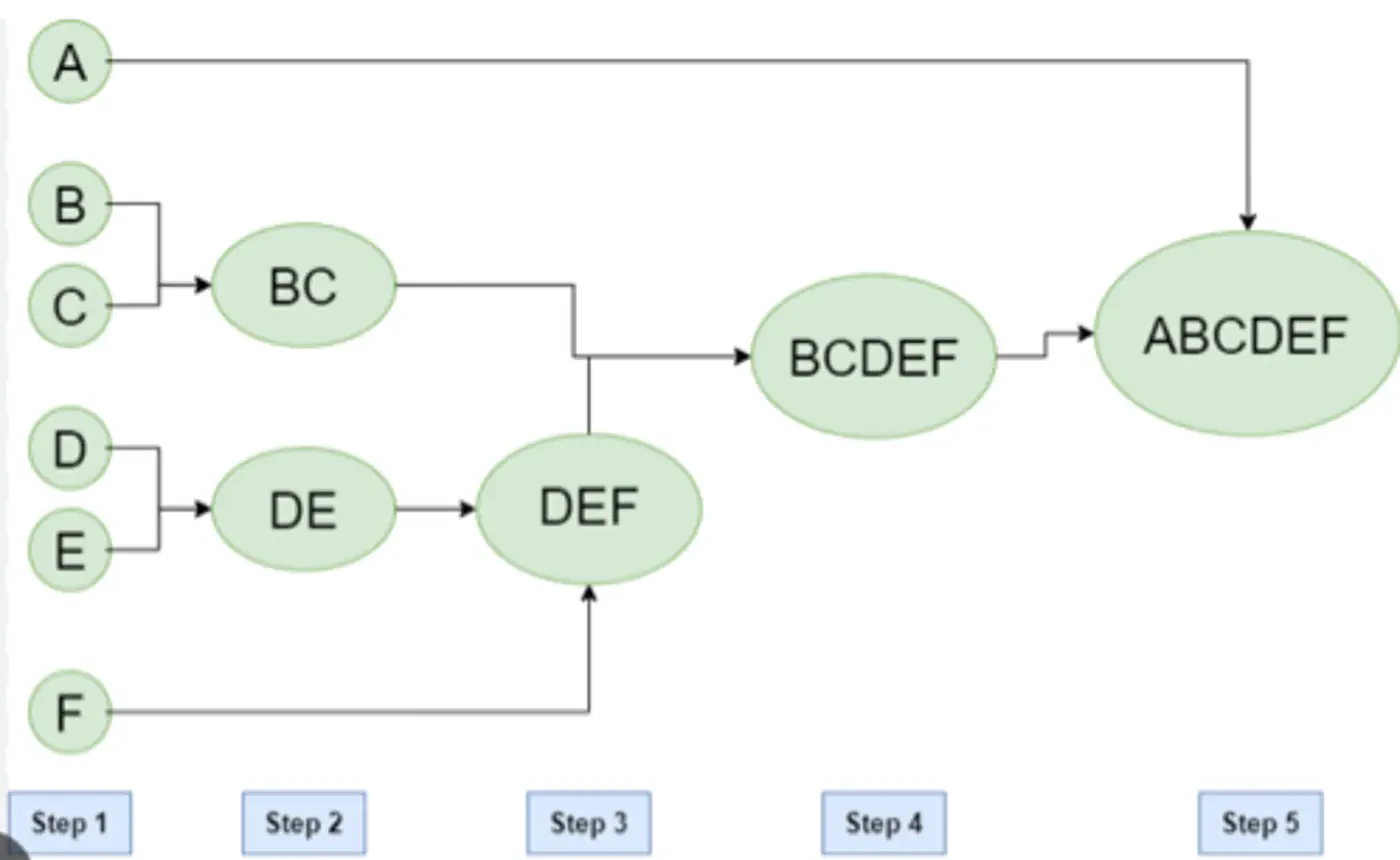
- Ward’s Method:
- Merges clusters to minimize the increase in the total within-cluster variance (sum of squared errors), resulting in compact, equally sized clusters.
- Single Linkage (MIN):
- Uses the minimum distance between any two points in different clusters.
- Prone to creating long, ‘chain-like’ 🔗 clusters, sensitive to outliers.
- Complete Linkage (MAX):
- Uses the maximum distance between any two points in different clusters.
- Forms tighter, more spherical clusters, less sensitive to outliers than single linkage.
- Average Linkage:
- Combines clusters by the average distance between all points in two clusters, offering a compromise between single and complete linkage.
- A good middle ground, often overcoming limitations of single and complete linkage.
- Centroid Method:
- Merges clusters based on the distance between their centroids (mean points).
👉Single Linkage is more sensitive to outlier than Complete Linkage, as Single Linkage can keep linking to the closest point forming a bridge to outlier.
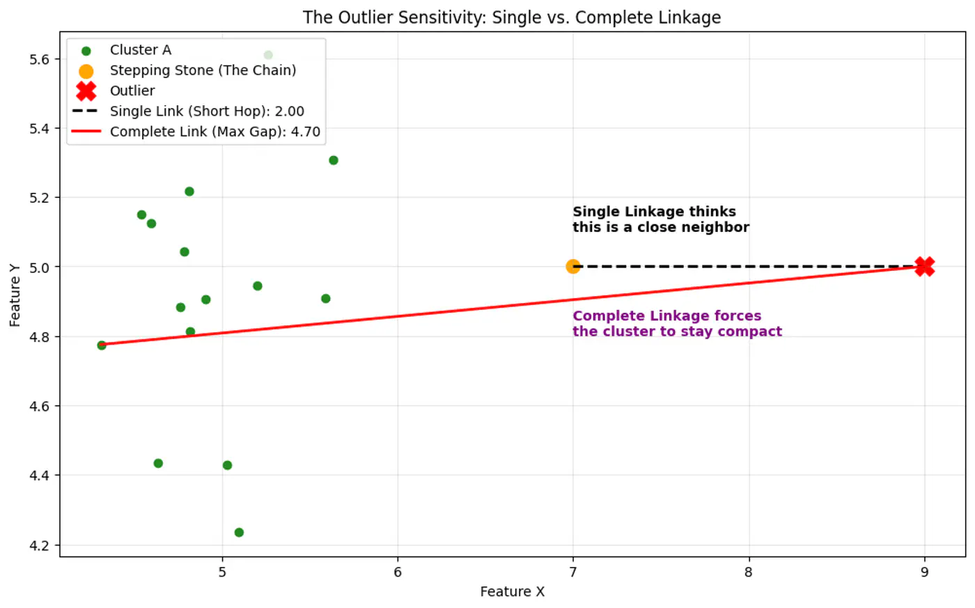
👉All cluster linkage distances.
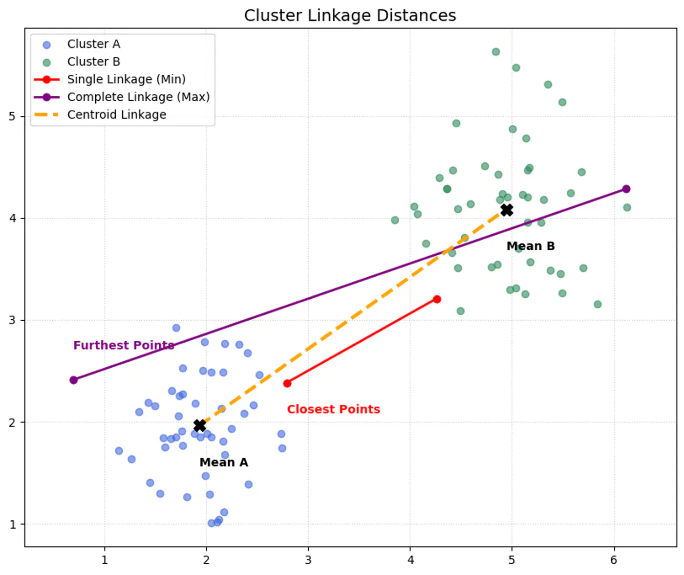
👉We get different clustering using different linkages.
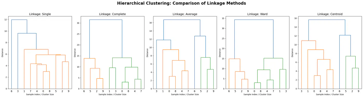
End of Section
3.3 - DBSCAN
3.3.1 - DBSCAN
- Non-Convex Shapes: K-Means can not find ‘crescent’ or ‘ring’ shape clusters.
- Noise: K-Means forces every point into a cluster, even outliers.
👉K-Means asks:
- “Which center is closest to this point?”
👉DBSCAN asks:
- “Is this point part of a dense neighborhood?”
⭐️Groups closely packed data points into clusters based on their density, and marks points that lie alone in low-density regions as outliers or noise.
Note: Unlike K-means, DBSCAN can find arbitrarily shaped clusters and does not require the number of clusters to be specified beforehand.
- Epsilon (eps or \(\epsilon\)):
- Radius that defines the neighborhood around a data point.
- If it’s too small, many points will be noise, and if too large, distinct clusters may merge.
- Minimum Points(minPts or min_samples):
- Minimum number of data points required within a point’s -neighborhood for that point to be considered a dense region (a core point).
- Defines threshold for ‘density’.
- Rule of thumb: minPts dimensions + 1; use larger value for noisy data (minPts 2*dimensions).
- Core Point:
- If it has at least minPts (including itself) within its -neighborhood.
- Forms the dense backbone of the clusters and can expand them.
- Border Point:
- If it has at fewer than minPts within its -neighborhood but falls within the -neighborhood of a core point.
- Border points belong to a cluster but cannot expand it further.
- Noise Point (Outlier):
- If it is neither a core point nor a border point, i.e., it is not density-reachable from any core point.
- Not assigned to any cluster.
- Random Start:
- Mark all points as unvisited; pick an arbitrary unvisited point ‘P’ from the dataset.
- Density Check:
- Check the point P’s ϵ-neighborhood.
- If ‘P’ has at least minPts, it is identified as a core point, and a new cluster is started.
- If it has fewer than minPts, the point is temporarily labeled as noise (it might become a border point later).
- Cluster Expansion:
- Recursively visit all points in P’s ϵ-neighborhood.
- If they are also core points, their neighbors are added to the cluster.
- Iteration 🔁:
- This ‘density-reachable’ logic continues until the cluster is fully expanded.
- The algorithm then picks another unvisited point and repeats the process, discovering new clusters or marking more points as noise until all points are processed.
👉DBSCAN can correctly detect non-spherical clusters.
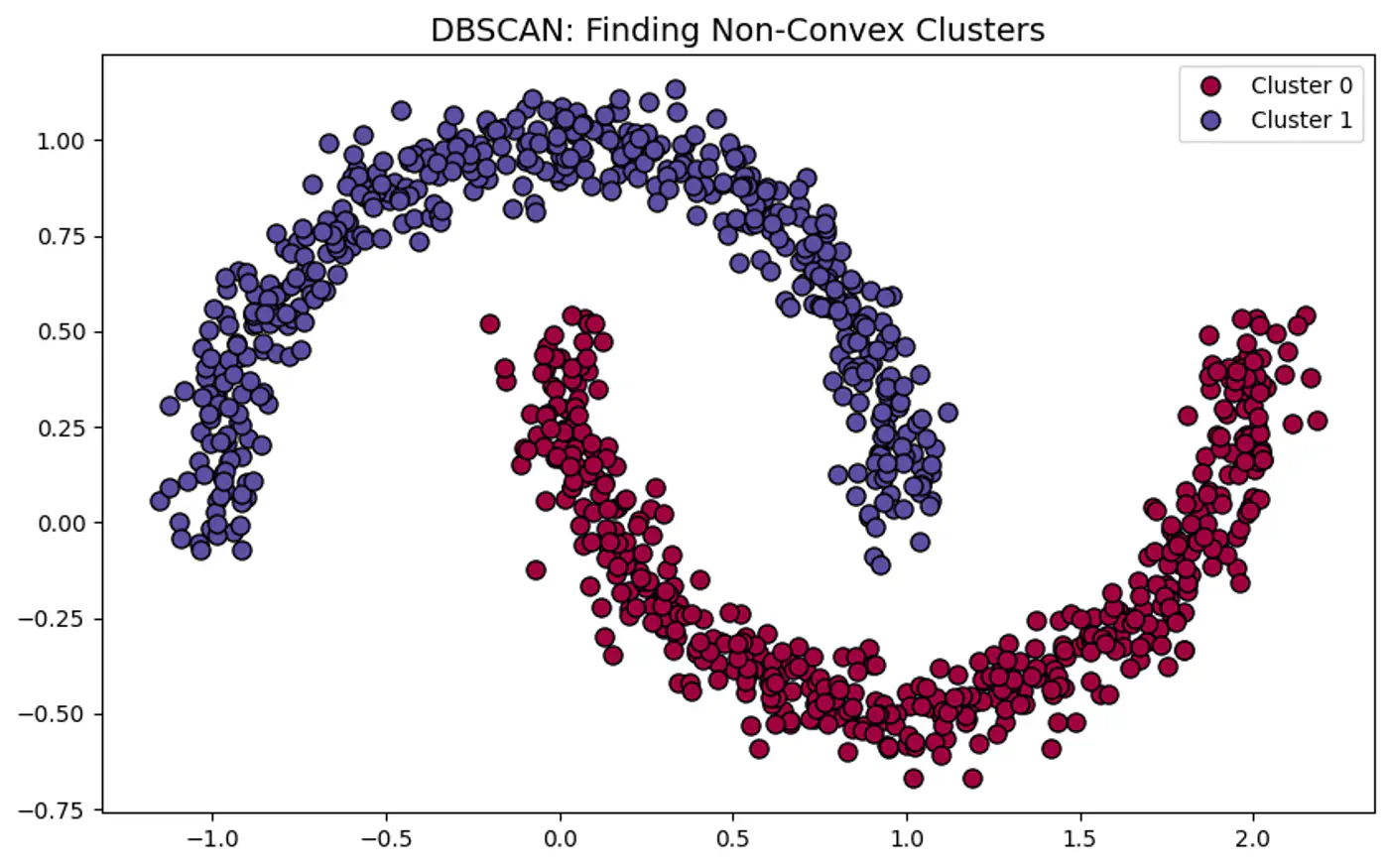
👉DBSCAN Points and Epsilon-Neighborhood.
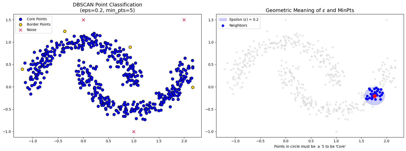
- Varying Density Clusters:
- Say A cluster is very dense and B is sparse, a single cannot satisfy both clusters.
- High Dimensional Data:
- ‘Curse of Dimensionality’ - In high-dimensional space, the distance between any two points converge.
Note: Sensitive to parameter eps and minPts; tricky to get it work.
👉DBSCAN Failure and Epsilon ((\epsilon)
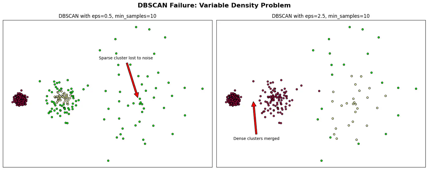
Arbitrary Cluster Shapes:
- When clusters are intertwined, nested, or ‘moon-shaped’; where K-Means would fail by splitting them.
Presence of Noise and Outliers:
- Robust to noise and outliers because it explicitly identifies low-density points as noise (labeled as -1) rather than forcing them into a cluster.
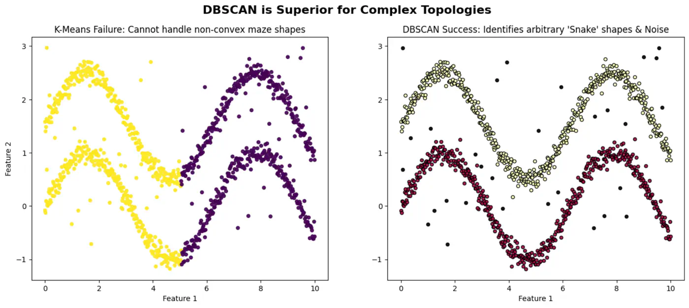
End of Section
3.4 - Gaussian Mixture Model
3.4.1 - Gaussian Mixture Models
- K-means uses Euclidean distance and assumes that clusters are spherical (isotropic) and have the same variance across all dimensions.
- Places a circle or sphere around each centroid.
- What if the clusters are elliptical ? 🤔
👉K-Means Fails with Elliptical Clusters.
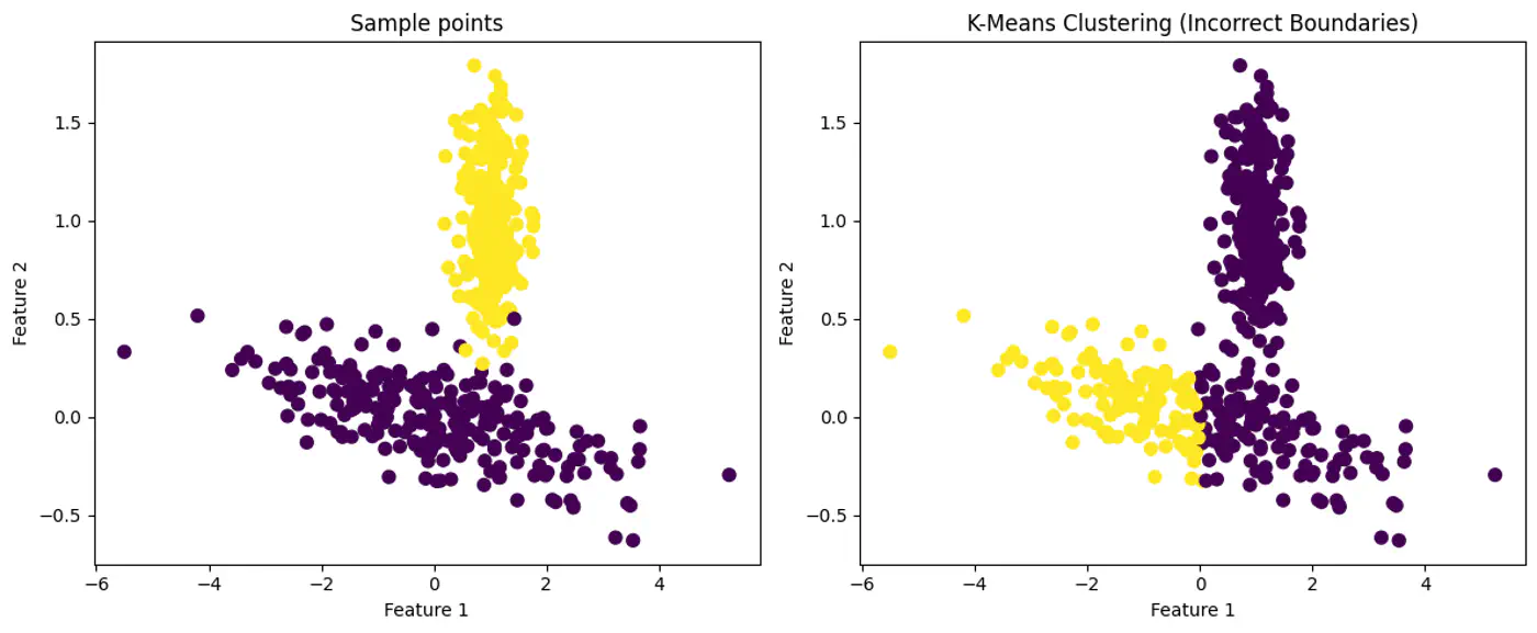
💡GMM: ‘Probabilistic evolution’ of K-Means
⭐️ GMM provides soft assignments and can model elliptical clusters by accounting for variance and correlation between features.
Note: GMM assumes that all data points are generated from a mixture of a finite number of Gaussian Distributions with unknown parameters.
👉GMM can Model Elliptical Clusters.
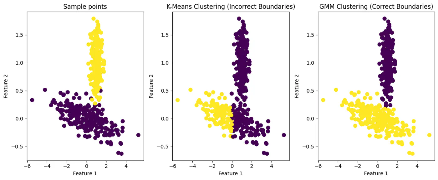
💡‘Combination of probability distributions’.
👉Soft Assignment: Instead of a simple ‘yes’ or ’no’ for cluster membership, a data point is assigned a set of probabilities, one for each cluster.
e.g: A data point might have a 60% probability of belonging to cluster ‘A’, 30% probability for cluster ‘B’, and 10% probability for cluster ‘C’.
👉Gaussian Mixture Model Example:
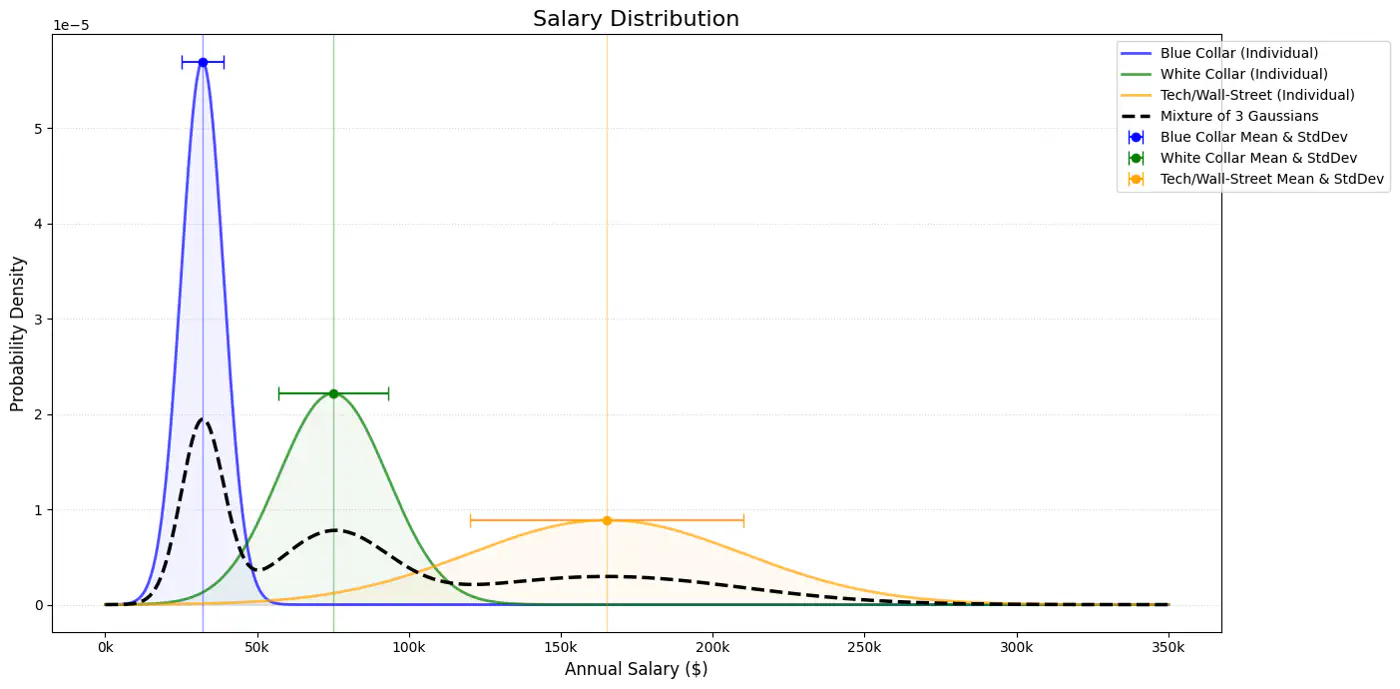
Note: The term \(1/(\sqrt{2\pi \sigma ^{2}})\) is a normalization constant to ensure the total area under the curve = 1.
👉Multivariate Gaussian Example:

Whenever we have multivariate Gaussian, then the variables may be independent or correlated.
👉Feature Covariance:
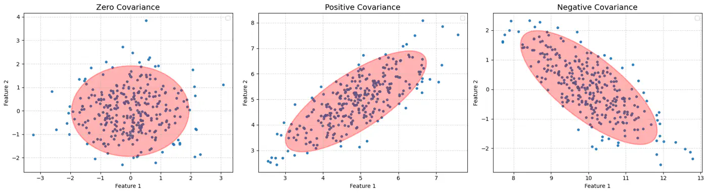
👉Gaussian Mixture with PDF
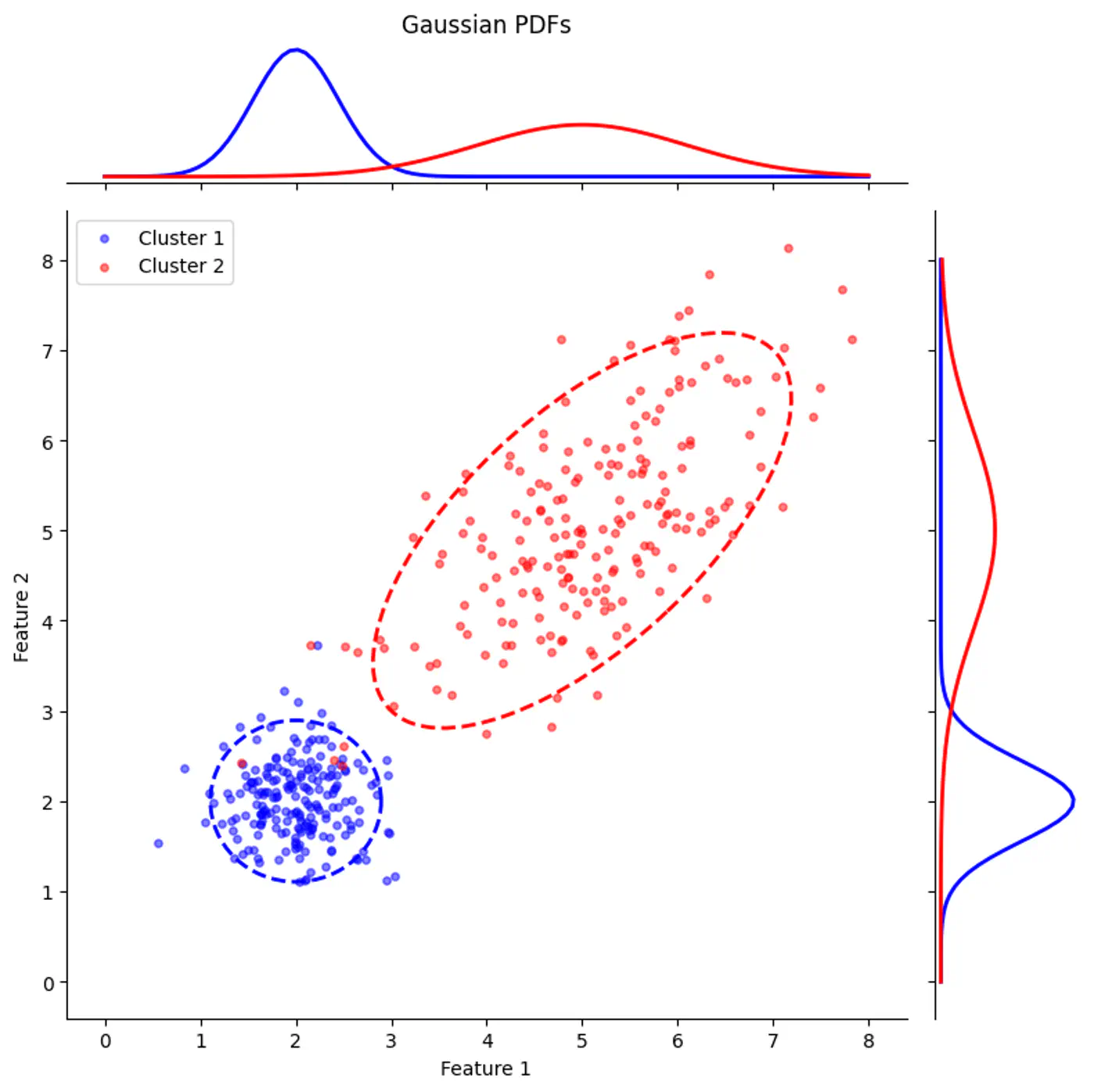
👉Gaussian Mixture (2D)
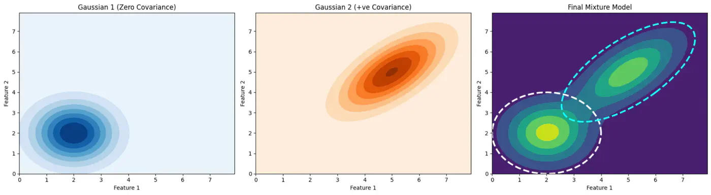
End of Section
3.4.2 - Latent Variable Model
⭐️Probabilistic model that assumes data is generated from a mixture of several Gaussian (normal) distributions with unknown parameters.
🎯GMM represents the probability density function of the data as a weighted sum of ‘K’ component Gaussian densities.
👉Below plot shows the probability of a point being generated by 3 different Gaussians.
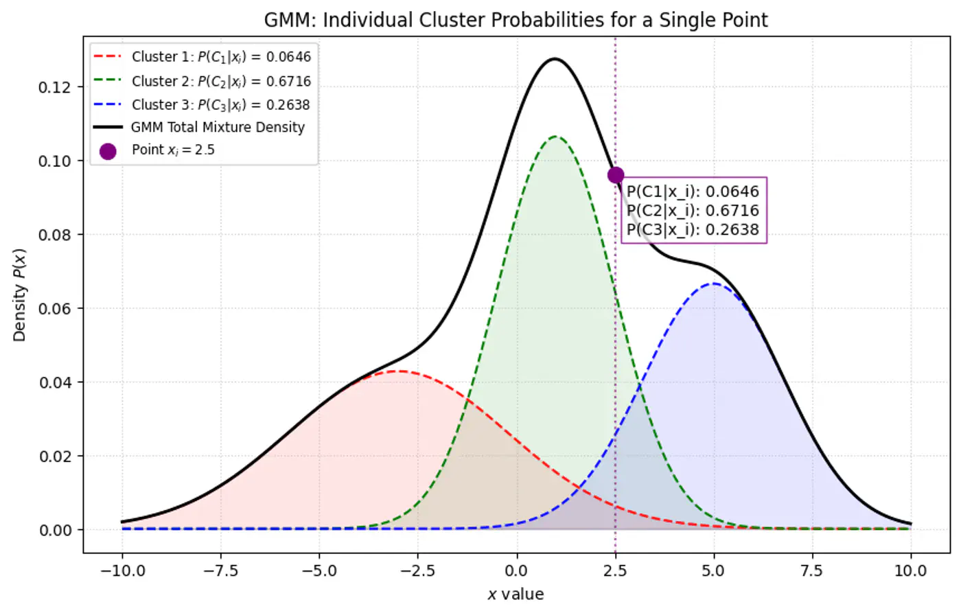
Overall density \(p(x_i|\mathbf{\theta })\) for a data point ‘\(x_i\)’:
\[p(x_i|\mathbf{\mu},\mathbf{\Sigma} )=\sum _{k=1}^{K}\pi _{k}\mathcal{N}(x_i|\mathbf{\mu }_{k},\mathbf{\Sigma }_{k})\]- K: number of component Gaussians.
- \(\pi_k\): mixing coefficient (weight) of the k-th component, such that, \(\pi_k \ge 0\) and \(\sum _{k=1}^{K}\pi _{k}=1\).
- \(\mathcal{N}(x_i|\mathbf{\mu }_{k},\mathbf{\Sigma }_{k})\): probability density function of the k-th Gaussian component with mean \(\mu_k\) and covariance matrix \(\Sigma_k\).
- \(\mathbf{\theta }=\{(\pi _{k},\mathbf{\mu }_{k},\mathbf{\Sigma }_{k})\}_{k=1}^{K}\): complete set of parameters to be estimated.
Note: \(\pi _{k}\approx \frac{\text{Number\ of\ points\ in\ cluster\ }k}{\text{Total\ number\ of\ points\ }(N)}\)
👉 Weight of the cluster is proportional to the number of points in the cluster.
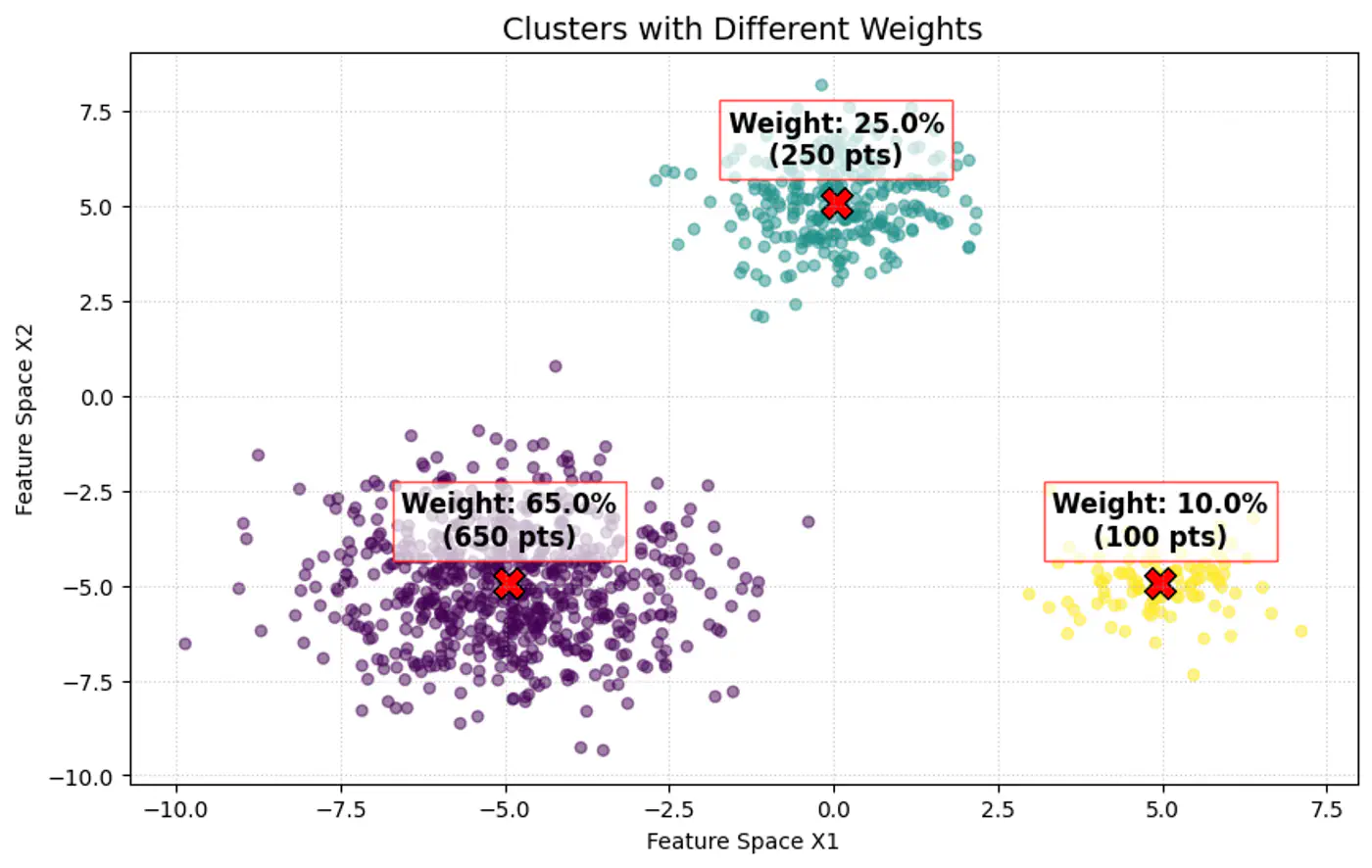
👉Below image shows the weighted Gaussian PDF, given the weights of clusters.
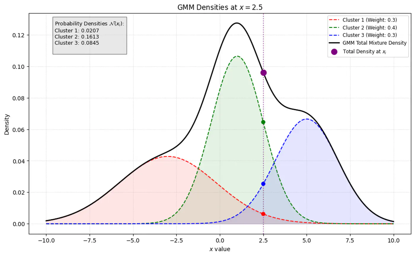
🎯 Goal of a GMM optimization is to find the set of parameters \(\Theta =\{(\pi _{k},\mu _{k},\Sigma _{k})\mid k=1,\dots ,K\}\) that maximize the likelihood of observing the given data.
\[L(\Theta |X)=\sum _{i=1}^{N}\log P(x_i|\Theta )=\sum _{i=1}^{N}\log \left(\sum _{k=1}^{K}\pi _{k}\mathcal{N}(x_i|\mu _{k},\Sigma _{k})\right)\]- 🦀 \(\log (A+B)\) cannot be simplified.
- 🦉So, is there any other way ?
⭐️Imagine we are measuring the heights of people in a college.
- We see a distribution with two peaks (bimodal).
- We suspect there are two underlying groups:
- Group A (Men) and Group B (Women).
Observation:
- Observed Variable (X): Actual height measurements.
- Latent Variable (Z): The ‘label’ (Man or Woman) for each person.
Note: We did not record gender, so it is ‘hidden’ or ‘latent’.
⭐️GMM is a latent variable model, meaning each data point \(\mathbf{x}_{i}\) is assumed to have an associated unobserved (latent) variable \(z_{i}\in \{1,\dots ,K\}\) indicating which component generated it.
Note: We observe the data point, but we do not observe which cluster it belongs to (\(z_i\)).
👉If we knew the value of \(z_i\) (component indicator) for every point, estimating the parameters of each Gaussian component would be straightforward.
Note: The challenge lies in estimating both the parameters of the Gaussians and the values of the latent variables simultaneously.
- With ‘z’ unknown:
- maximize: \[ \log \sum _{k}\pi _{k}\mathcal{N}(x_{i}|\mu _{k},\Sigma _{k}) = \log \Big(\pi _{1}\mathcal{N}(x_{i}\mid \mu _{1},\Sigma _{1})+\pi _{2}\mathcal{N}(x_{i}\mid \mu _{2},\Sigma _{2})+ \dots + \pi _{k}\mathcal{N}(x_{i}\mid \mu _{k},\Sigma _{k})\Big)\]
- \(\log (A+B)\) cannot be simplified.
- maximize: \[ \log \sum _{k}\pi _{k}\mathcal{N}(x_{i}|\mu _{k},\Sigma _{k}) = \log \Big(\pi _{1}\mathcal{N}(x_{i}\mid \mu _{1},\Sigma _{1})+\pi _{2}\mathcal{N}(x_{i}\mid \mu _{2},\Sigma _{2})+ \dots + \pi _{k}\mathcal{N}(x_{i}\mid \mu _{k},\Sigma _{k})\Big)\]
- With ‘z’ known:
- The log-likelihood of the ‘complete data’ simplifies into a sum of logarithms:
\[\sum _{i}\log (\pi _{z_{i}}\mathcal{N}(x_{i}|\mu _{z_{i}},\Sigma _{z_{i}}))\]
- Every point is assigned to exactly one cluster, so the sum disappears because there is only one cluster responsible for that point.
- The log-likelihood of the ‘complete data’ simplifies into a sum of logarithms:
\[\sum _{i}\log (\pi _{z_{i}}\mathcal{N}(x_{i}|\mu _{z_{i}},\Sigma _{z_{i}}))\]
Note: This allows the logarithm to act directly on the exponential term of the Gaussian, leading to simple linear equations.
👉When ‘z’ is known, every data point is ‘labeled’ with its parent component.
To estimate the parameters (mean \(\mu_k\) and covariance \(\Sigma_k\)) for a specific component ‘k’ :
- Gather all data points \(x_i\), where \(z_i\)= k.
- Calculate the standard Maximum Likelihood Estimate.(MLE) for that single Gaussian using only those points.
⭐️ Knowing ‘z’ provides exact counts and component assignments, leading to direct formulae for the parameters:
- Mean (\(\mu_k\)): Arithmetic average of all points assigned to component ‘k’.
- Covariance (\(\Sigma_k\)): Sample covariance of all points assigned to component ‘k’.
- Mixing Weight (\(\pi_k\)): Fraction of total points assigned to component ‘k’.
End of Section
3.4.3 - Expectation Maximization
- If we knew the parameters (\(\mu, \Sigma, \pi\)) we could easily calculate which cluster ‘z’ each point belongs to (using probability).
- If we knew the cluster assignments ‘z’ of each point, we could easily calculate the parameters for each cluster (using simple averages).
🦉But we do not know either of them, as the parameters of the Gaussians - we aim to find and cluster indicator latent variable is hidden.
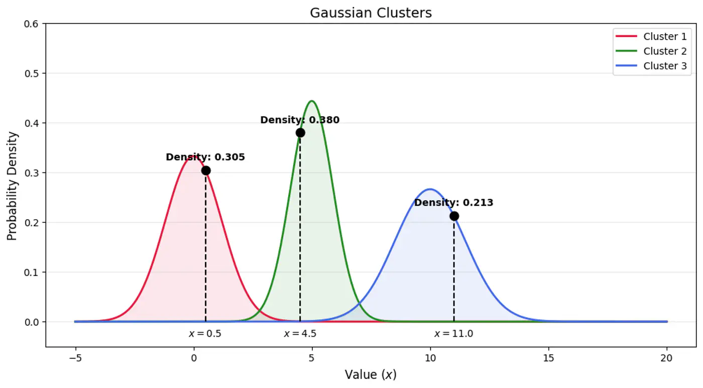

⛳️ Find latent cluster indicator variable \(z_{ik}\).
But \(z_{ik}\) is a ‘hard’ assignment’ (either ‘0’ or ‘1’).
- 🦆 Because we do not observe ‘z’, we use another variable ‘Responsibility’ (\(\gamma_{ik}\)) as a ‘soft’ assignment (value between 0 and 1).
- 🐣 \(\gamma_{ik}\) is the expected value of the latent variable \(z_{ik}\), given the observed data \(x_{i}\) and parameters \(\Theta\). \[\gamma _{ik}=E[z_{ik}\mid x_{i},\theta ]=P(z_{ik}=1\mid x_{i},\theta )\]
Note: \(\gamma_{ik}\) is the posterior probability (or ‘responsibility’) that cluster ‘k’ takes for explaining data point \(x_{i}\).
⭐️Using Bayes’ Theorem, we derive responsibility (posterior probability that component ‘k’ generated data point \(x_i\)) by combining the prior/weights (\(\pi_k\)) and the likelihood (\(\mathcal{N}(x_{i}\mid \mu _{k},\Sigma _{k})\)).
\[\gamma _{ik}= P(z_{ik}=1\mid x_{i},\theta ) = \frac{P(z_{ik}=1)P(x_{i}\mid z_{ik}=1)}{P(x_{i})}\]\[\gamma _{ik}=\frac{\pi _{k}\mathcal{N}(x_{i}\mid \mu _{k},\Sigma _{k})}{\sum _{j=1}^{K}\pi _{j}\mathcal{N}(x_{i}\mid \mu _{j},\Sigma _{j})}\]👉Bayes’ Theorem: \(P(A|B)=\frac{P(B|A)\cdot P(A)}{P(B)}\)
👉 GMM Densities at point
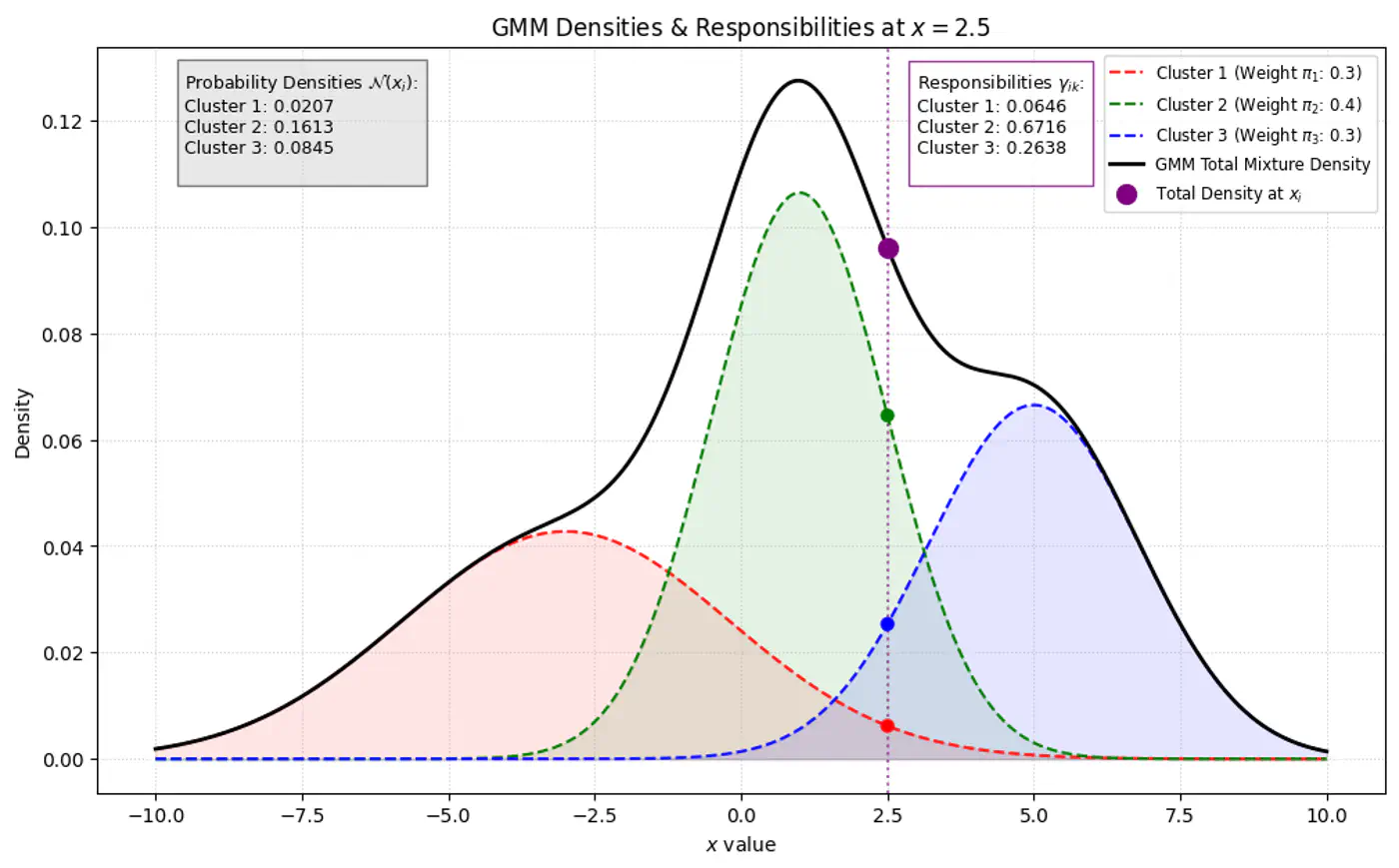
👉GMM Densities at point (different cluster weights)
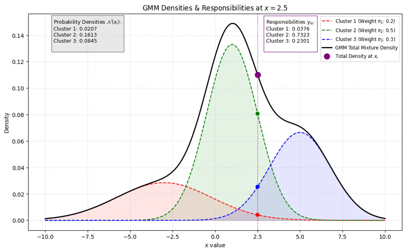
- Initialization: Assign initial values to parameters (\(\mu, \Sigma, \pi\)), often using K-Means results.
- Expectation Step (E): Calculate responsibilities; provides ‘soft’ assignments of points to clusters.
- Maximization Step (M): Update parameters using responsibilities as weights to maximize the expected log-likelihood.
- Convergence: Repeat ‘E’ and ‘M’ steps until the change in log-likelihood falls below a threshold.
👉Given our current guess of the clusters, what is the probability that point \(x_i\) came from cluster ‘k’ ?
\[\gamma (z_{ik})=p(z_{i}=k|\mathbf{x}_{i},\mathbf{\theta }^{(\text{old})})=\frac{\pi _{k}^{(\text{old})}\mathcal{N}(\mathbf{x}_{i}|\mathbf{\mu }_{k}^{(\text{old})},\mathbf{\Sigma }_{k}^{(\text{old})})}{\sum _{j=1}^{K}\pi _{j}^{(\text{old})}\mathcal{N}(\mathbf{x}_{i}|\mathbf{\mu }_{j}^{(\text{old})},\mathbf{\Sigma }_{j}^{(\text{old})})}\]\(\pi_k\) : Probability that a randomly selected data point \(x_i\) belongs to the k-th component before we even look at the specific value of \(x_i\), such that \(\pi_k \ge 0\) and \(\sum _{k=1}^{K}\pi _{k}=1\).
👉Update the parameters (\(\mu, \Sigma, \pi\)) by calculating weighted versions of the standard MLE formulas using responsibilities as weight 🏋️♀️.
\[ \begin{align*} &\bullet \mathbf{\mu }_{k}^{(\text{new})}=\frac{1}{N_{k}}\sum _{i=1}^{N}\gamma (z_{ik})\mathbf{x}_{i} \\ &\bullet \mathbf{\Sigma }_{k}^{(\text{new})}=\frac{1}{N_{k}}\sum _{i=1}^{N}\gamma (z_{ik})(\mathbf{x}_{i}-\mathbf{\mu }_{k}^{(\text{new})})(\mathbf{x}_{i}-\mathbf{\mu }_{k}^{(\text{new})})^{\top } \\ &\bullet \pi _{k}^{(\text{new})}=\frac{N_{k}}{N} \end{align*} \]- where, \(N_{k}=\sum _{i=1}^{N}\gamma (z_{ik})\) is the effective number of points assigned to component ‘k'.
End of Section
3.5.1 - Anomaly Detection
🦄 Anomaly is a rare item, event or observation which deviates significantly from the majority of the data and does not conform to a well-defined notion of normal behavior.
Note: Such examples may arouse suspicions of being generated by a different mechanism, or appear inconsistent with the remainder of that set of data.
❌ Remove Outliers:
- Rejection or omission of outliers from the data to aid statistical analysis, for example to compute the mean or standard deviation of the dataset.
- Remove outliers for better predictions from models, such as linear regression.
🔦Focus on Outliers:
- Fraud detection in banking and financial services.
- Cyber-security: intrusion detection, malware, or unusual user access patterns.
- Supervised
- Semi-Supervised
- Unsupervised (most common) ✅
Note: Labeled anomaly data is often unavailable in real-world scenarios.
- Statistical Methods: Z-Score, large value means outlier, IQR, point beyond fences (Q1 - 1.5*IQR or Q3 + 1.5*IQR) is flagged as an outlier.
- Distance Based: KNN, points far from their neighbors as potential anomalies.
- Density Based: DBSCAN, points in low density regions are considered outliers.
- Clustering Based: K-Means, points far from cluster centroids that do not fit any cluster are anomalies.
- Elliptic Envelope (MCD - Minimum Covariance Determinant)
- One-Class SVM (OC-SVM)
- Local Outlier Factor (LOF)
- Isolation Forest (iForest)
- RANSAC (Random Sample Consensus)
End of Section
3.5.2 - Elliptic Envelope
Detect anomalies in multivariate Gaussian data, such as, biometric data (height/weight) where features are normally distributed and correlated.
Assumption: The data can be modeled by a Gaussian distribution.
In a normal distribution, most data points cluster around the mean, and the probability density decreases as we move farther away from the center.
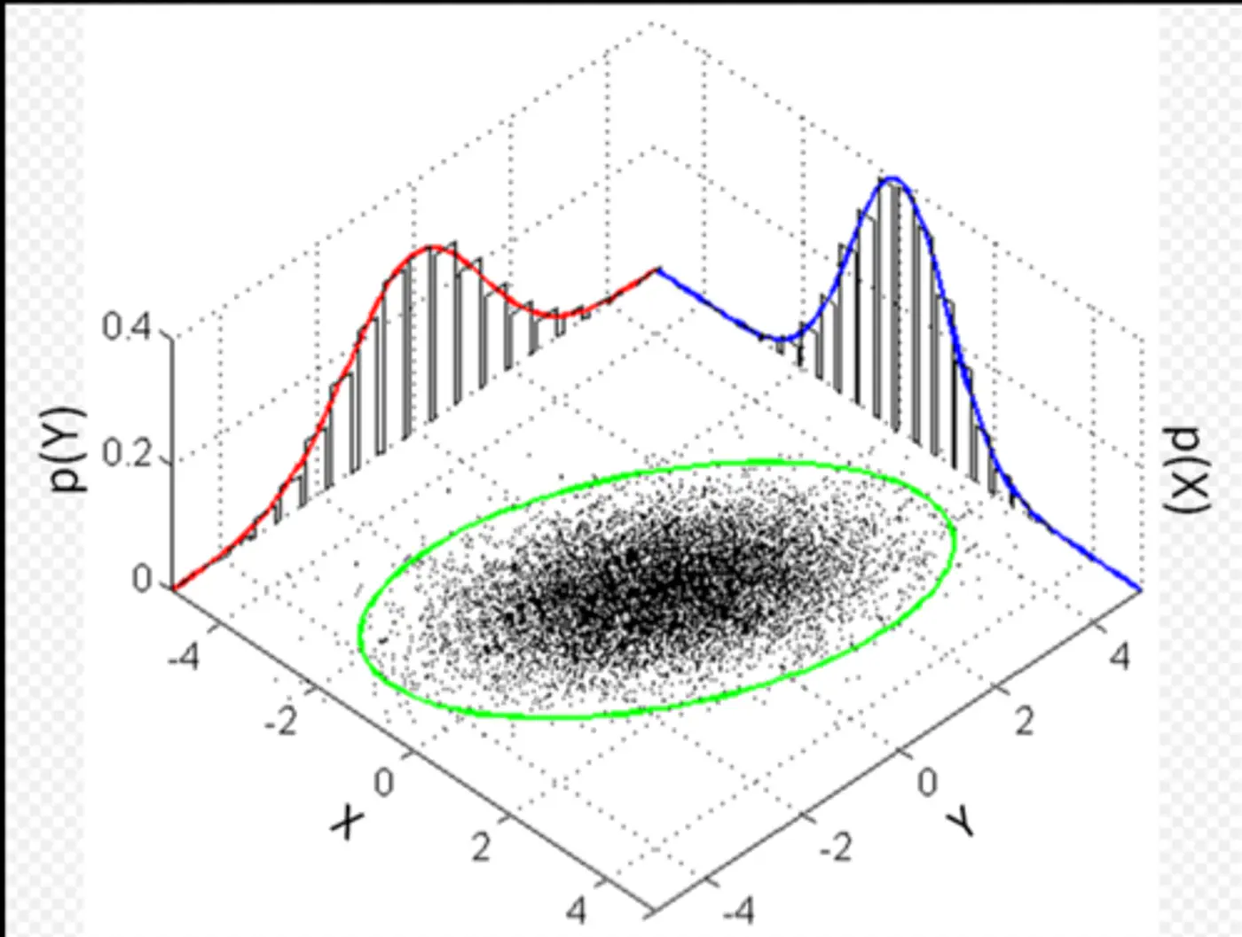
🌍 Euclidean distance measures the simple straight-line distance from the center of the cloud.
👉If the data is spherical, this works fine.
🦕 However, real-world data is often stretched or skewed (e.g., taller people are generally heavier), due to correlations between variables, forming an elliptical shape.

⭐️Mahalanobis distance essentially re-scales the data so that the elliptical distribution appears spherical, and then measures the Euclidean distance in that transformed space.
👉This way, it measures how many standard deviations(\(\sigma\)) away a point is from the mean, considering the data’s spread and correlation (covariance).
\[D_M(x) = \sqrt{(x - \mu)^T \Sigma^{-1} (x - \mu)}\]👉Find the most dense core of the data.
\[D_M(x) = \sqrt{(x - \mu)^T \Sigma^{-1} (x - \mu)}\]🦣 Determinant of covariance matrix \(\Sigma\) represents the volume of the ellipsoid.
⏲️ Therefore, minimize \(|\Sigma|\) to find the tight core.
👉 \(\text {Small} ~ \Sigma \rightarrow \text {Large} ~\Sigma ^{-1}\rightarrow \text {Large} ~ D_{M} ~\text {for outliers}\)
MCD algorithm is used to find the covariance matrix \(\Sigma\) with minimum determinant, so that the volume of the ellipsoid is minimized.
- Initialization: Select several random subsets of size h < n (default h = \(\frac{n+d+1}{2}\), d = # dimensions), representing ‘robust’ majority of the data.
- Calculate preliminary mean (\(\mu\)) and covariance (\(\Sigma\)) for each random subset.
- Concentration Step: Iterative core of the algorithm designed to ‘tighten’ the ellipsoid.
- Calculate Distances: Compute the Mahalanobis distance of all ’n’ points in the dataset from the current subset’s mean (\(\mu\)) and covariance (\(\Sigma\)).
- Select New Subset: Identify the ‘h’ points with the smallest Mahalanobis distances.
- These are the points most centrally located relative to the current ellipsoid.
- Update Estimates: Calculate a new and based only on these ‘h’ most central points.
- Repeat 🔁: The steps repeat until the determinant stops shrinking.
Note: Select the best subset that achieved the absolute minimum determinant.
- Assumptions
- Gaussian data.
- Unimodal data (single center).
- Cost 💰of covariance matrix \(\Sigma^{-1}\) inversion is O(d^3).
End of Section
3.5.3 - One Class SVM
⭐️Only one class of data (normal, non-outlier) is available for training, making standard supervised learning models impossible.
e.g. Only normal observations are available for fraud detection, cyber attack, fault detection etc.

🦂 The core problem is to build a model that can distinguish between ‘normal’ and ‘anomalous’ data when we only have examples of the ‘normal’ class during training.
🦖 We need to find a decision boundary that is as compact as possible while still encompassing the bulk of the training data.
🦍 Define a boundary for a single class in high-dimensional space where data might be non-linearly distributed (e.g.‘U’ shape).
🦧 Use the Kernel Trick to project data into a higher-dimensional space and find a hyperplane that separates the data from the origin with the maximum margin.
⭐️OC-SVM, as introduced by Bernhard Schölkopf et al., uses a hyperplane ‘H’ defined by a weight vector \(\mathbf{w}\) and a bias term \(\rho\).
👉Solve the following optimization problem:
\[\min _{\mathbf{w},\xi _{i},\rho }\frac{1}{2}||\mathbf{w}||^{2}+\frac{1}{\nu N}\sum _{i=1}^{N}\xi _{i}-\rho \]Subject to constraints:
\[\mathbf{w}\cdot \phi (\mathbf{x}_{i})\ge \rho -\xi _{i}\quad \text{and}\quad \xi _{i}\ge 0,\quad \text{for\ }i=1,\dots ,N\]- \(\mathbf{x}_{i}\): i-th training data point.
- \(\phi (\mathbf{x}_{i})\): RBF kernel function \(K(x, y) = \exp(-\gamma \|x-y\|^2)\) that maps the data into a higher-dimensional feature space, making it easier to separate from the origin.
- \(\mathbf{w}\): normal vector to the separating hyperplane.
- \(\rho\): scalar bias term that determines the offset of the hyperplane from the origin.
- \(\xi_i\): Slack variables that allow some data points to fall on the ‘wrong’ side of the hyperplane (inside the anomalous region) to prevent overfitting.
- N: total number of training points.
- \(\nu\): hyper-parameter between 0 and 1. It acts as an upper bound on the fraction of outliers (training data points outside the boundary) and a lower bound on the fraction of support vectors.
- \(\frac{1}{2}\|\mathbf{w}\|^{2}\): aims to maximize the margin/compactness of the region.
- \(\frac{1}{\nu N}\sum _{i=1}^{N}\xi _{i}-\rho\): penalizes points (outliers) that violate the boundary constraints.
After solving the optimization problem using standard quadratic programming techniques, we obtain the optimal \(\mathbf{w}^{*}\) and \(\rho ^{*}\).
For a new data point \(x_{new}\), decision function is:
\[f(\mathbf{x}_{\text{new}})=\text{sign}(\mathbf{w}^{*}\cdot \phi (\mathbf{x}_{\text{new}})-\rho ^{*})\]\(f(\mathbf{x}_{\text{new}})\ge 0\): normal point.
\(f(\mathbf{x}_{\text{new}})< 0\): anomalous point (outlier).
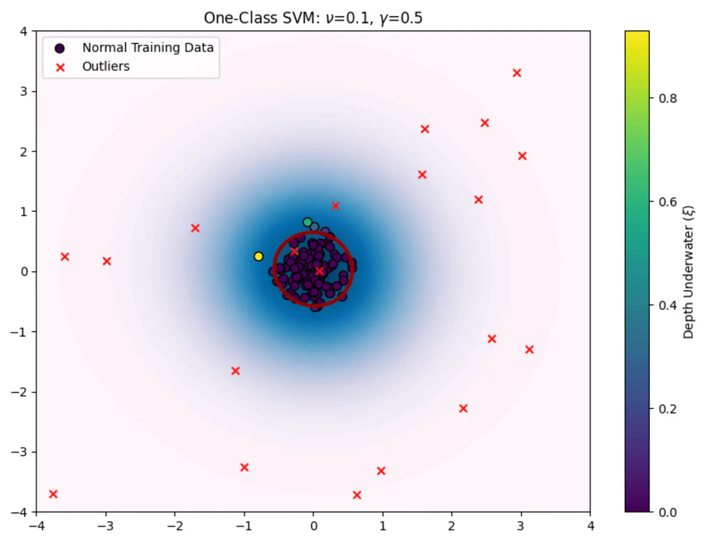
End of Section
3.5.4 - Local Outlier Factor
A $100 transaction might be ‘normal’ in New York but an ‘outlier’ in a small rural village.
‘Local context matters.’
Global distance metrics fail when density is non-uniform.
🦄 An outlier is a point that is ‘unusual’ relative to its immediate neighbors, regardless of how far it is from the center of the entire dataset.
💡Traditional distance-based outlier detection methods, such as, KNN, often struggle with datasets where data is clustered at varying densities.
- A point in a sparse region might be considered an outlier by a global method, even if it is a normal part of that sparse cluster.
- Conversely, a point very close to a dense cluster might be an outlier relative to that specific neighborhood.
👉Calculate the relative density of a point compared to its immediate neighborhood.
e.g. If the neighbors are in a dense crowd and the point is not, it is an outlier.
Local Outlier Factor (LOF) is a density-based algorithm designed to detect anomalies by measuring the local deviation of a data point relative to its neighbors.
👉Size of the red circle represents the LOF score.
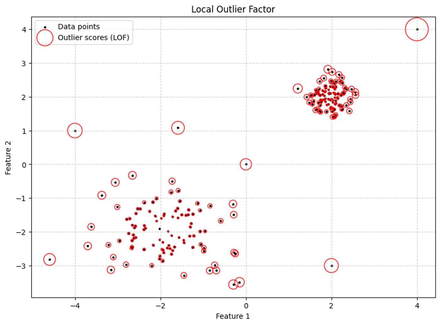
- K-Distance (\(k\text{-dist}(p)\)):
- The distance from point ‘p’ to its k-th nearest neighbor.
- Reachability Distance (\(\text{reach-dist}_{k}(p,o)\)):
\[\text{reach-dist}_{k}(p,o)=\max \{k\text{-dist}(o),\text{dist}(p,o)\}\]
- \(\text{dist}(p,o)\): actual Euclidean distance between ‘p’ and ‘o’.
- This acts as ‘smoothing’ factor.
- If point ‘p’ is very close to ‘o’ (inside o’s k-neighborhood), round up distance to \(k\text{-dist}(o)\).
- \(\text{dist}(p,o)\): actual Euclidean distance between ‘p’ and ‘o’.
- Local Reachability Density (\(\text{lrd}_{k}(p)\)):
- The inverse of the average reachability distance from ‘p’ to its k-neighbors (\(N_{k}(p)\)).
\[\text{lrd}_{k}(p)=\left[\frac{1}{|N_{k}(p)|}\sum _{o\in N_{k}(p)}\text{reach-dist}_{k}(p,o)\right]^{-1}\]
- High LRD: Neighbors are very close; the point is in a dense region.
- Low LRD: Neighbors are far away; the point is in a sparse region.
- The inverse of the average reachability distance from ‘p’ to its k-neighbors (\(N_{k}(p)\)).
\[\text{lrd}_{k}(p)=\left[\frac{1}{|N_{k}(p)|}\sum _{o\in N_{k}(p)}\text{reach-dist}_{k}(p,o)\right]^{-1}\]
- Local Outlier Factor (\(\text{LOF}_{k}(p)\)):
- The ratio of the average ‘lrd’ of p’s neighbors to p’s own ‘lrd’. \[\text{LOF}_{k}(p)=\frac{1}{|N_{k}(p)|}\sum _{o\in N_{k}(p)}\frac{\text{lrd}_{k}(o)}{\text{lrd}_{k}(p)}\]
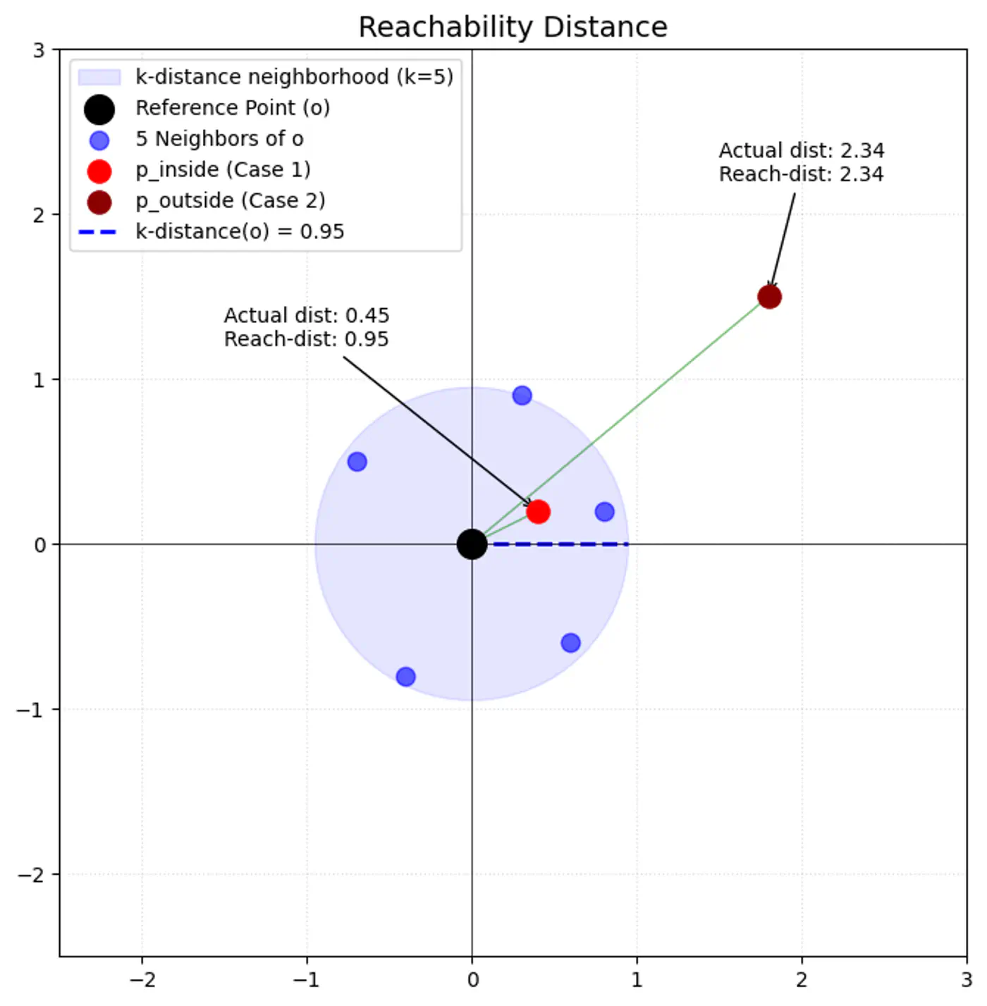
- LOF ≈ 1: Point ‘p’ has similar density to its neighbors (inlier).
- LOF > 1: Point p’s density is much lower than its neighbors’ density (outlier).
End of Section
3.5.5 - Isolation Forest
‘Large scale tabular data.’
Credit card fraud detection in datasets with millions of rows and hundreds of features.
Note: Supervised learning requires balanced, labeled datasets (normal vs. anomaly), which are rarely available in real-world scenarios like fraud or cyber-attacks.
🦥 ‘Flip the logic.’
🦄 ‘Anomalies’ are few and different, so they are much easier to isolate from the rest of the data than normal points.
🐦🔥 ‘Curse of dimensionality.’
🐎 Distance based (K-NN), and density based (LOF) algorithms require calculation of distance between all pair of points.
🐙 As the number of dimensions and data points grows, these calculations become exponentially more expensive 💰 and less effective.
‘Randomly partition the data.’
🦄 If a point is an outlier, it will take fewer partitions (splits) to isolate it into a leaf 🍃 node compared to a point that is buried deep within a dense cluster of normal data.
🌳Isolation Forest uses an ensemble of ‘Isolation Trees’ (iTrees) 🌲.
👉iTree (Isolation Tree) 🌲 is a proper binary tree structure specifically designed to separate individual data points through random recursive partitioning.
- Sub-sampling:
- Select a random subset of data (typically 256 instances) to build an iTree.
- Tree Construction: Randomly select a feature.
- Randomly select a split value between the minimum and maximum values of that feature.
- Divide the data into two branches based on this split.
- Repeat recursively until the point is isolated or a height limit is reached.
- Forest Creation:
- Repeat 🔁 the process to create ‘N’ trees (typically 100).
- Inference:
- Pass a new data point through all trees, calculate the average path length, and compute the anomaly score.
⭐️🦄 Assign an anomaly score based on the path length h(x) required to isolate a point ‘x’.
- Path Length (h(x)): The number of edges ‘x’ traverses from the root node to a leaf node.
- Average Path Length (c(n)): Since iTrees are structurally similar to Binary Search Trees (BST), the average path length for a dataset of size ’n’ is given by: \[c(n)=2H(n-1)-\frac{2(n-1)}{n}\]
where, H(i) is the harmonic number, estimated as \(\ln (i)+0.5772156649\) (Euler’s constant).
To normalize the score between 0 and 1, we define it as:
\[s(x,n)=2^{-\frac{E(h(x))}{c(n)}}\]👉E(H(x)): is the average path length of across a forest of trees 🌲.
- \(s\rightarrow 1\): Point is an anomaly; Path length is very short.
- \(s\approx 0.5\): Point is normal, path length approximately equal to c(n).
- \(s\rightarrow 0\): Point is normal; deeply buried point, path length is much larger than c(n).
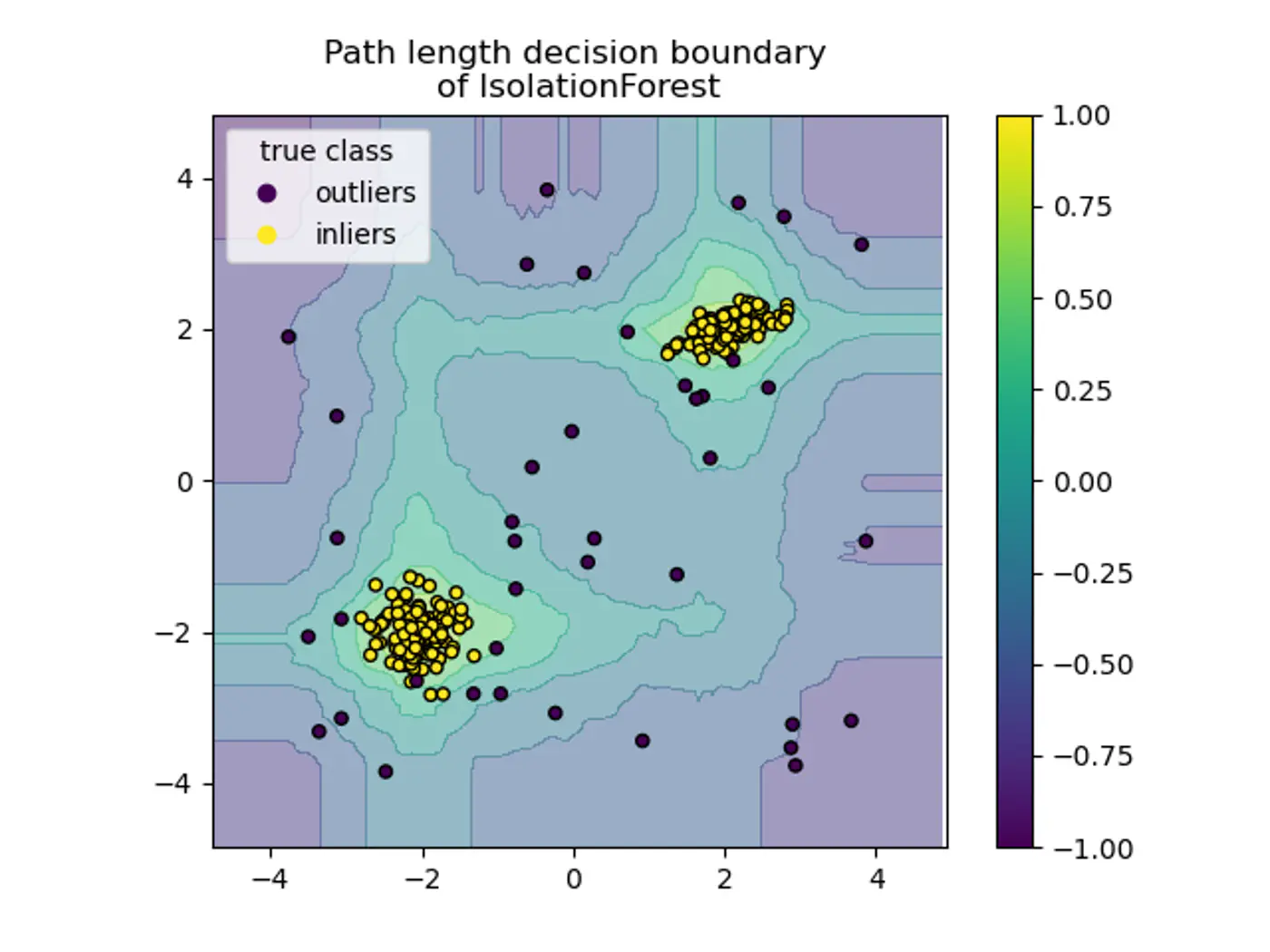
- Axis-Parallel Splits:
- Standard iTrees 🌲 split only on one feature at a time, so:
- We do not get a smooth decision boundary.
- Anything off-axis has a higher probability of being marked as an outlier.
- Note: Extended Isolation Forest fixes this by using random slopes.
- Standard iTrees 🌲 split only on one feature at a time, so:
- Score Sensitivity: The threshold for what constitutes an ‘anomaly’ often requires manual tuning or domain knowledge.
End of Section
3.5.6 - RANSAC
👉Ordinary Least Squares use all data points to find a fit.
- However, a single outlier can ‘pull’ the resulting line significantly, leading to a poor representative model.
💡If we pick a very small random subset of points, there is a higher probability that this small subset contains only good data (inliers) compared to a large set.
Ordinary Least Squares (OLS) minimizes the Sum of Errors.
- A huge outlier has an exponentially large impact on the final line.
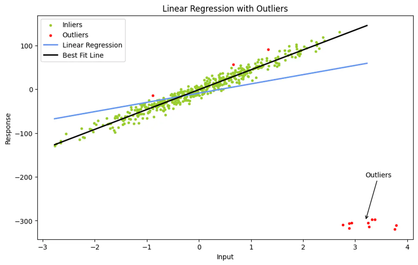
💡Instead of using all points, iteratively pick the smallest possible random subset to fit a model, then check (votes) how many other points in the dataset ‘agree’ with that model.
This gives the name to our algorithm:
- Random: Random subsets.
- Sampling: Small subsets.
- Consensus: Agreement with other points.
- Random Sampling:
- Randomly select a Minimal Sample Set (MSS) of ’n’ points from the input data ‘D’.
- e.g. n=2 for a line, or n=3 for a plane in 3D.
- Model Fitting:
- Compute the model parameters using only these ’n’ points.
- Test:
- For all other points in ‘D’, calculate the error relative to the model.
- 👉 Points with error < \(\tau\)(threshold) are added to the ‘Consensus Set’.
- Evaluate:
- If the consensus set is larger than the previous best, save this model and set.
- Repeat 🔁:
- Iterate ‘k’ times.
- Refine (Optional):
- Once the best model is found, re-estimate it using all points in the final consensus set (usually via Least Squares) for a more precise fit.
👉Example:
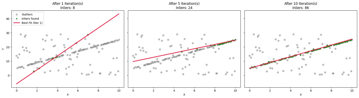
👉To ensure the algorithm finds a ‘clean’ sample set (no outliers) with a desired probability(often 99%), we use the following formula:
\[k=\frac{\log (1-P)}{\log (1-w^{n})}\]- k: Number of iterations required.
- P: Probability that at least one random sample contains only inliers.
- w: Ratio of inliers in the dataset (number of inliers / total points).
- n: Number of points in the Minimal Sample Set.
End of Section
3.6 - Dimensionality Reduction
3.6.1 - PCA
- Data Compression
- Noise Reduction
- Feature Extraction: Create a smaller set of meaningful features from a larger one.
- Data Visualization: Project high-dimensional data down to 2 or 3 dimensions.
Assumption: Linear relationship between features.
💡‘Information = Variance’
☁️ Imagine a cloud of points in 2D space.
👀 Look for the direction (axis) along which the data is most ‘spread out’.
🚀 By projecting data onto this axis, we retain the maximum amount of information (variance).
👉Example 1: Var(Feature 1) < Var(Feature 1)
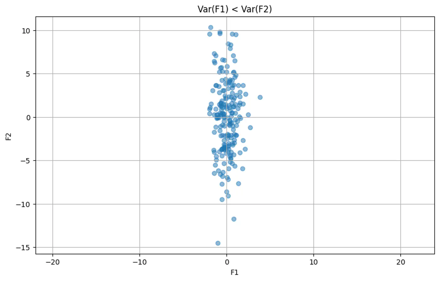
👉Example 2: Red line shows the direction of maximum variance
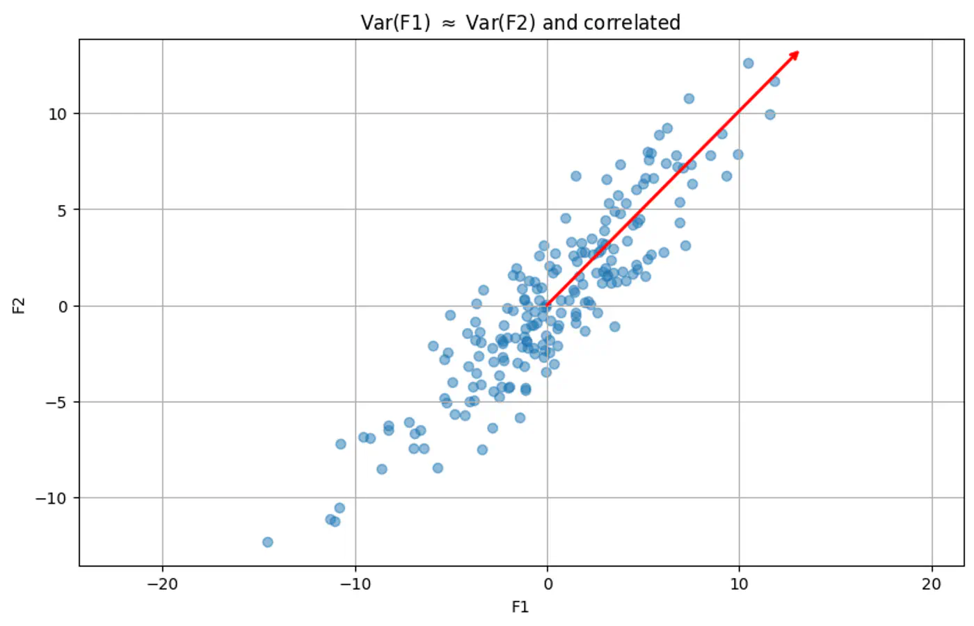
🧭 Finds the direction of maximum variance in the data.
Note: Some loss of information will always be there in dimensionality reduction, because there will be some variability in data along the direction that is dropped, and that will be lost.
- PCA seeks a direction 🧭, represented by a unit vector \(\hat{u}\) onto which data can be projected to maximize variance.
- The projection of a mean centered data point \(x_i\) onto \(u\) is \(u^Tx_i\).
- The variance of these projections can be expressed as \(u^{T}\Sigma u\), where \(\Sigma\) is the data’s covariance matrix.
- Data: Let \(X = \{x_{1},x_{2},\dots ,x_{n}\}\) is the mean centered (\(\bar{x} = 0\)) dataset.
- Projection of point \(x_i\) on \(u\) is \(z_i = u^Tx_i\)
- Variance of projected points (since \(\bar{x} = 0\)): \[\text{Var}(z)=\frac{1}{n}\sum _{i=1}^{n}z_{i}^{2}=\frac{1}{n}\sum _{i=1}^{n}(x_{i}^{T}u)^{2}\]
- 💡Since, \((x_{i}^{T}u)^{2} = (u^{T}x_{i})(x_{i}^{T}u)\) \( \implies\text{Var}(z)=u^{T}\left(\frac{1}{n}\sum _{i=1}^{n}x_{i}x_{i}^{T}\right)u\)
- 💡Since, Covariance Matrix, \(\Sigma = \left(\frac{1}{n}\sum _{i=1}^{n}x_{i}x_{i}^{T}\right)\)
- 👉 Therefore, \(\text{Var}(z)=u^{T}\Sigma u\)
👉 To prevent infinite variance, PCA constrains \(u\) to be a unit vector (\(\|u\|=1\)).
\[\text{maximize\ }u^{T}\Sigma u, \quad \text{subject\ to\ }u^{T}u=1\]Note: This constraint forces the optimization algorithm to focus purely on the direction that maximizes variance, rather than allowing it to artificially inflate the variance by increasing the length of the vector.
⏲️ Lagrangian function: \(L(u,\lambda )=u^{T}\Sigma u-\lambda (u^{T}u-1)\)
🔦 To find \(u\) that maximizes above constrained optimization:
💎 This is the standard Eigenvalue Equation.
🧭 So, the optimal directions \(u\) are the eigenvectors of the covariance matrix \(\Sigma\).
👉 To see which eigenvector maximizes variance, substitute the result back into the variance equation:
\[\text{Variance}=u^{T}\Sigma u=u^{T}(\lambda u)=\lambda (u^{T}u)=\lambda \]🧭 Since the variance equals the eigenvalue \(\lambda\), the direction \(u\) that maximizes variance is the eigenvector associated with the largest eigenvalue.
- Center the data: \(X = X - \mu\)
- Compute the Covariance Matrix: \(\Sigma = \frac{1}{n-1} X^T X\)
- Compute Eigenvectors and Eigenvalues of \(\Sigma\) .
- Sort eigenvalues in descending order and select the top ‘k’ eigenvectors.
- Project the original data onto the subspace: \(Z = X W_k\) where, \(W_{k}=[u_{1},u_{2},\dots ,u_{k}]\) , matrix formed by ‘k’ eigenvectors corresponding to ‘k’ largest eigenvalues.
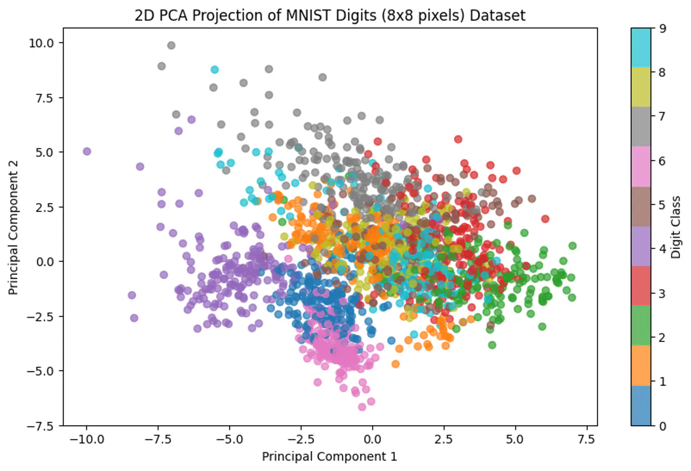
- Cannot model non-linear relationships.
- Sensitive to outliers.
End of Section
3.6.2 - t-SNE
👉 PCA preserves variance, not neighborhoods.
🔬 t-SNE focuses on the ‘neighborhood’ (local structure).
💡Tries to keep points that are close together in high-dimensional space close together in low-dimensional space.
👉 Map high-dimensional points to low-dimensional points , such that the pairwise similarities are preserved, while solving the ‘crowding problem’ (where points collapse into a single cluster).
👉 Crowding Problem
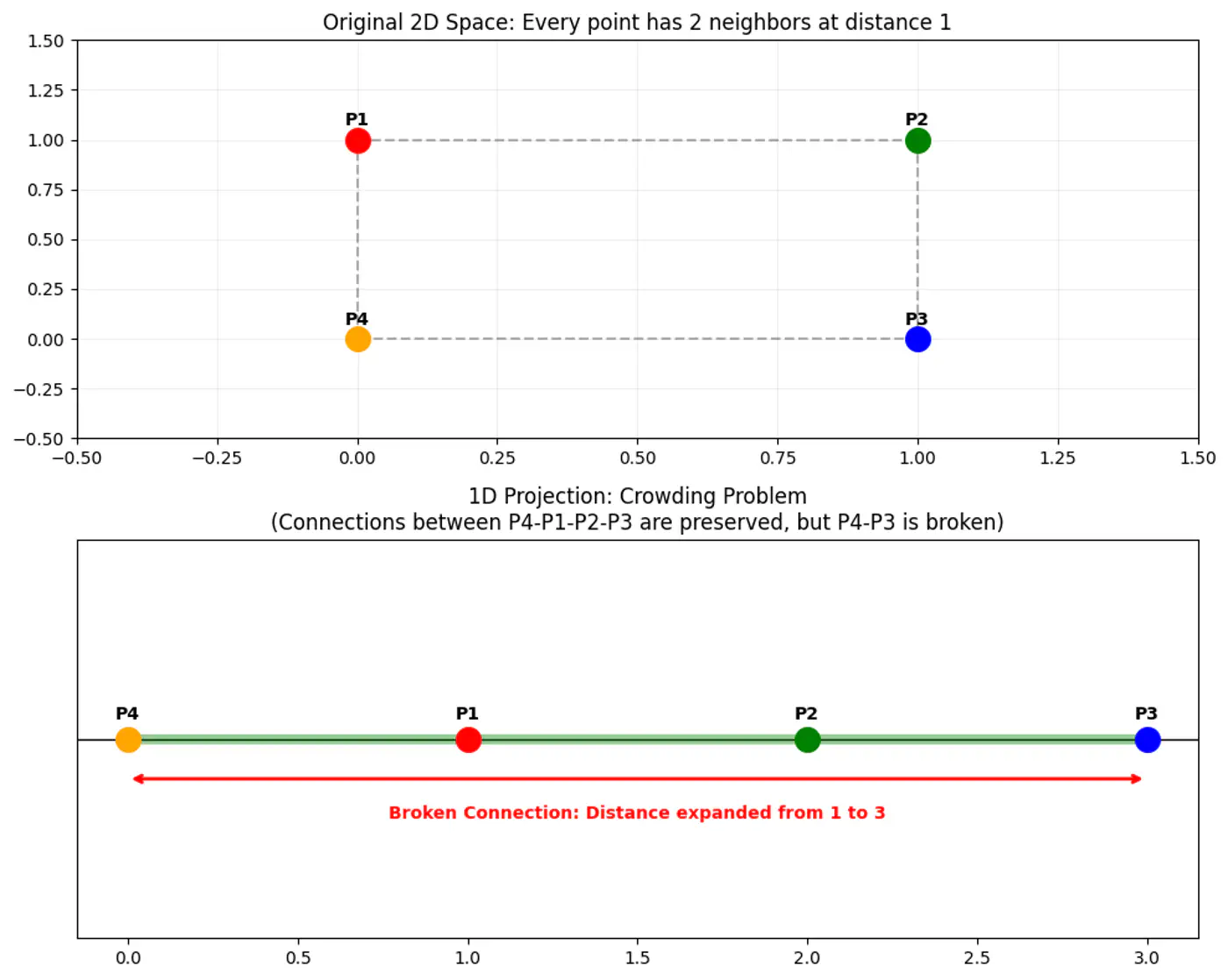
📌 Convert Euclidean distances into conditional probabilities representing similarities.
⚖️ Minimize the divergence between the probability distributions of the high-dimensional (Gaussian)
and low-dimensional (t-distribution) spaces.
Note: Probabilistic approach to defining neighbors is the core ‘stochastic’ element of the algorithm’s name.
💡The similarity of datapoint \(x_j\) to datapoint \(x_i\) is the conditional probability \(p_{j|i}\), that \(x_i\) would pick \(x_j\) as its neighbor.
Note: If neighbors are picked in proportion to their probability density under a Gaussian centered at \(x_i\).
\[p_{j|i} = \frac{\exp(-||x_i - x_j||^2 / 2\sigma_i^2)}{\sum_{k \neq i} \exp(-||x_i - x_k||^2 / 2\sigma_i^2)}\]- \(p_{j|i}\) high: nearby points.
- \(p_{j|i}\) low: widely separated points.
Note: Make probabilities symmetric: \(p_{ij} = \frac{p_{j|i} + p_{i|j}}{2n}\)
🧠 To solve the crowding problem, we use a heavy-tailed 🦨 distribution (Student’s-t distribution with degree of freedom \(\nu=1\)).
\[q_{ij} = \frac{(1 + ||y_i - y_j||^2)^{-1}}{\sum_{k \neq l} (1 + ||y_k - y_l||^2)^{-1}}\]Note: Heavier tail spreads out dissimilar points more effectively, allowing moderately distant points to be mapped further apart, preventing clusters from collapsing and ensuring visual separation and cluster distinctness.
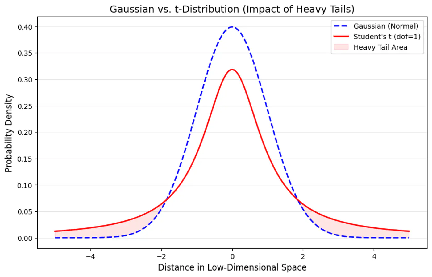
👉 Measure the difference between the distributions ‘p’ and ‘q’ using the Kullback-Leibler (KL) divergence, which we aim to minimize:
\[C = KL(P||Q) = \sum_i \sum_j p_{ij} \log \frac{p_{ij}}{q_{ij}}\]🏔️ Use gradient descent to iteratively adjust the positions of the low-dimensional points \(y_i\).
👉 The gradient of the KL divergence is:
\[\frac{\partial C}{\partial y_{i}}=4\sum _{j\ne i}(p_{ij}-q_{ij})(y_{i}-y_{j})(1+||y_{i}-y_{j}||^{2})^{-1}\]- C : t-SNE cost function (sum of all KL divergences).
- \(y_i, y_j\): coordinates of data points and in the low-dimensional space (typically 2D or 3D).
- \(p_{ij}\): high-dimensional similarity (joint probability) between points \(x_i\) and \(x_j\), calculated using a Gaussian distribution.
- \(q_{ij}\): low-dimensional similarity (joint probability) between points \(y_i\) and \(y_j\), calculated using a Student’s t-distribution with one degree of freedom.
- \((1+||y_{i}-y_{j}||^{2})^{-1}\): term comes from the heavy-tailed Student’s t-distribution, which helps mitigate the ‘crowding problem’ by allowing points that are moderately far apart to have a small attractive force.
💡 The gradient can be understood as a force acting on each point \(y_i\) in the low-dimensional map:
\[\frac{\partial C}{\partial y_{i}}=4\sum _{j\ne i}(p_{ij}-q_{ij})(y_{i}-y_{j})(1+||y_{i}-y_{j}||^{2})^{-1}\]- Attractive forces: If \(p_{ij}\) is large ⬆️ and \(q_{ij}\) is small ⬇️ (meaning two points were close in the high-dimensional space but are far in the low-dimensional space), the term \((p_{ij}-q_{ij})\) is positive, resulting in a strong attractive force pulling \(y_i\) and \(y_j\) closer.
- Repulsive forces: If \(p_{ij}\) is small ⬇️ and \(q_{ij}\) is large ⬆️ (meaning two points were far in the high-dimensional space but are close in the low-dimensional space), the term \((p_{ij}-q_{ij})\) is negative, resulting in a repulsive force pushing \(y_i\) and \(y_j\) apart.
👉 Update step of in low dimensions:
\[y_{i}^{(t+1)}=y_{i}^{(t)}-\eta \frac{\partial C}{\partial y_{i}}\]Attractive forces (\(p_{ij}>q_{ij}\)):
- The negative gradient moves \(y_i\) opposite to the (\(y_i - y_j\)) vector, pulling it toward \(y_j\).
Repulsive forces (\(p_{ij} < q_{ij}\)):
- The negative gradient moves \(y_i\) in the same direction as the (\(y_i - y_j\)) vector, pushing it away from \(y_j\).
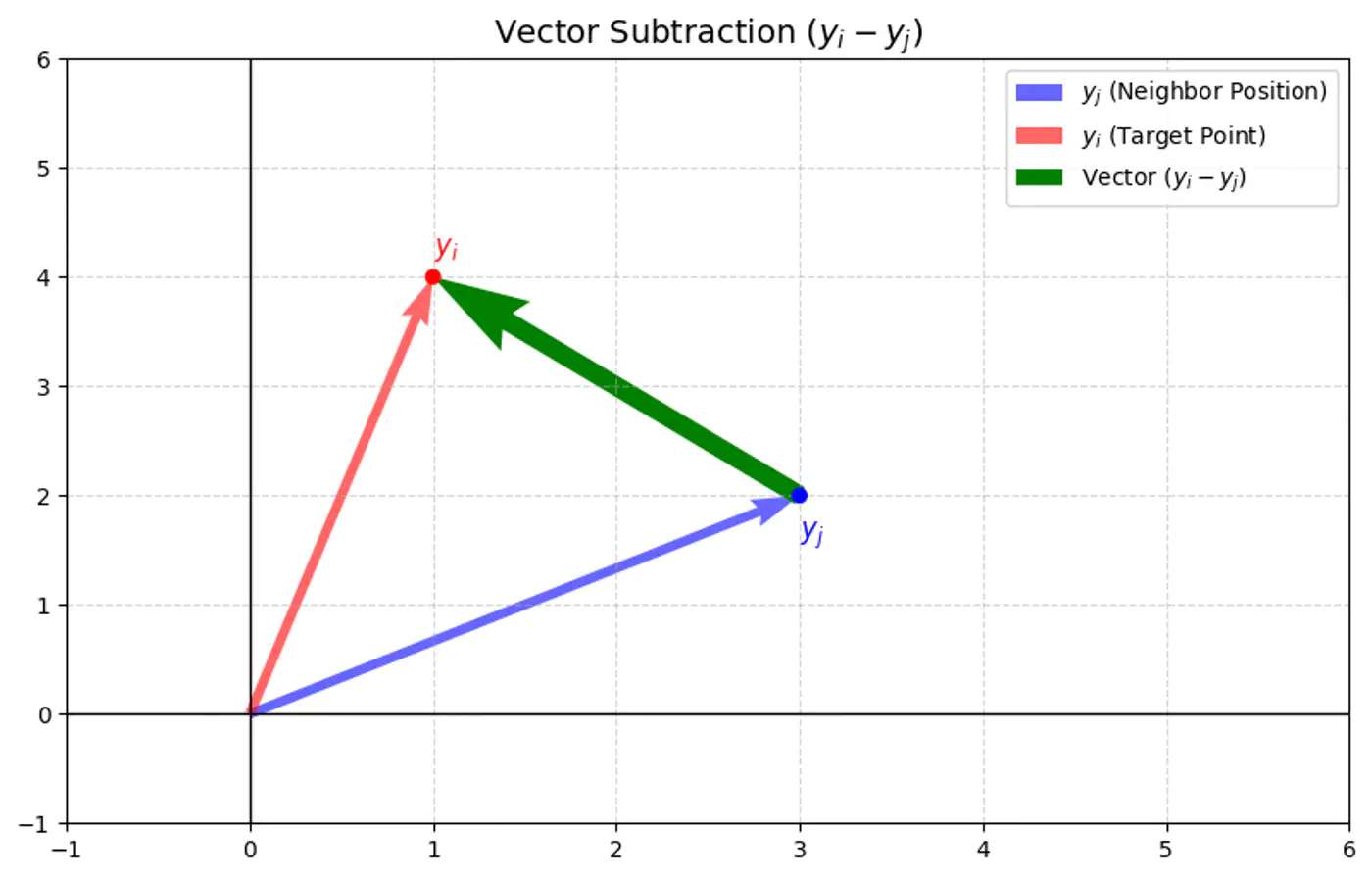
🏘️ User-defined parameter that loosely relates to the effective number of neighbors.
Note: Variance \(\sigma_i^2\) (Gaussian) is adjusted for each point to maintain a consistent perplexity.
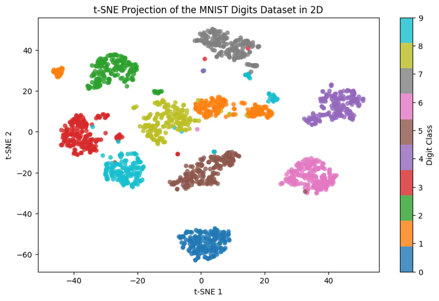
End of Section
3.6.3 - UMAP
🐢Visualizing massive datasets where t-SNE is too slow.
⭐️ Creating robust low-dimensional inputs for subsequent machine learning models.
⭐️ Using a world map 🗺️ (2D)instead of globe 🌍 for spherical(3D) earth 🌏.
👉It preserves the neighborhood relationships of countries (e.g., India is next to China), and to a good degree, the global structure.
⭐️ Non-linear dimensionality reduction technique to visualize high-dimensional data (like images, gene expressions)
in a lower-dimensional space (typically 2D or 3D), preserving its underlying structure and relationships.
👉 Constructs a high-dimensional graph of data points and then optimizes a lower-dimensional layout to closely match this graph, making complex datasets understandable by revealing patterns, clusters, and anomalies.
Note: Similar to t-SNE but often faster and better at maintaining global structure.
💡 Create a weighted graph (fuzzy simplicial set) representing the data’s topology and then find a low-dimensional graph that is as structurally similar as possible.
Note: Fuzzy means instead of using binary 0/1, we use weights in the range [0,1] for each edge.
- UMAP determines local connectivity based on a user-defined number of neighbors (n_neighbors).
- Normalizes distances locally using the distance to the nearest neighbor (\(\rho_i\)) and a scaling factor (\(\sigma_i\)) adjusted to enforce local connectivity constraints.
- The weight \(W_{ij}\) (fuzzy similarity) in high-dimensional space is: \[W_{ij}=\exp \left(-\frac{\max (0,\|x_{i}-x_{j}\|-\rho _{i})}{\sigma _{i}}\right)\]
Note: This ensures that the closest point always gets a weight of 1, preserving local structure.
👉In the low-dimensional space (e.g., 2D), UMAP uses a simple curve (similar to the t-distribution used in t-SNE) for edge weights:
\[Z_{ij}=(1+a\|y_{i}-y_{j}\|^{2b})^{-1}\]Note: The parameters ‘a’ and ‘b’ are typically fixed based on the ‘min_dist’ user parameter (e.g. min_dist = 0.1, then a≈1,577, b≈0.895).
⭐️ Unlike t-SNE’s KL divergence, UMAP minimizes the cross-entropy between the high-dimensional weights \(W_{ij}\) and the low-dimensional weights \(Z_{ij}\).
👉 Cost 💰 Function (C):
\[C=\sum _{i,j}\left(W_{ij}\log \frac{W_{ij}}{Z_{ij}}+(1-W_{ij})\log \frac{1-W_{ij}}{1-Z_{ij}}\right)\]Cost 💰 Function (C):
\[C=\sum _{i,j}\left(W_{ij}\log \frac{W_{ij}}{Z_{ij}}+(1-W_{ij})\log \frac{1-W_{ij}}{1-Z_{ij}}\right)\]🎯 Goal : Reduce overall Cross Entropy Loss.
- Attractive Force: \(W_{ij}\) high; make \(Z_{ij}\) high to make the log \(\frac{W_{ij}}{Z_{ij}} \)term small.
- Repulsive Force: \(W_{ij}\) low; make \(Z_{ij}\) low to make the \(log\frac{1-W_{ij}}{1-Z_{ij}}\) term small.
Note: This push and pull of 2 ‘forces’ will make the data in low dimensions settle into a position that is overall a good representation of the original data in higher dimensions.
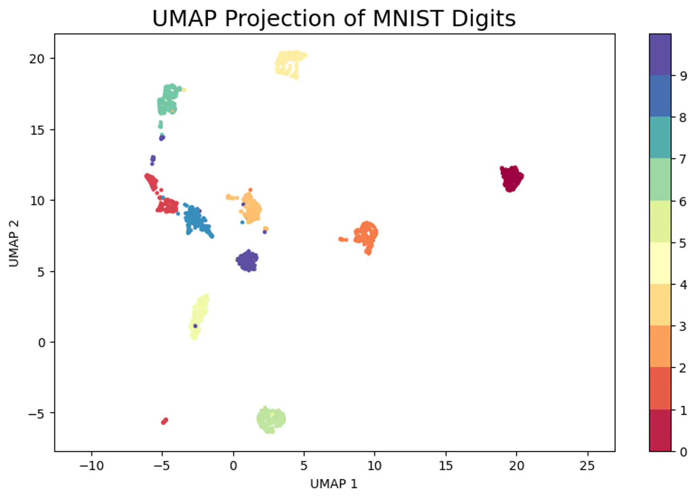
- Mathematically complex.
- Requires tuning (n_neighbors, min_dist).
End of Section
4.1 - Data Pre Processing
Messy and Incomplete.
We need to pre-process the data to make it:
- Clean
- Consistent
- Mathematically valid
- Computationally stable
👉 So that, the machine learning algorithm can safely consume the data.
- Missing Completely At Random (MCAR)
- The missingness occurs entirely by chance, such as due to a technical glitch during data collection or a random human error in data entry.
- Missing At Random (MAR)
- The probability of missingness depends on the observed data and not on the missing value itself.
- e.g. In some survey, the age of many females are missing, because they may not like to disclose the information.
- Missing Not At Random (MNAR)
- The probability of missingness is directly related to the unobserved missing value itself.
- e.g. Individuals with very high incomes 💰may intentionally refuse to report their salary due to privacy concerns, making the missing data directly dependent on the high income 💰value itself.
- Simple Imputation:
- Mean: Normally distributed numerical features.
- Median: Skewed numerical features.
- Mode: Categorical features, most frequent.
- KNN Imputation:
- Replace the missing value with mean/median/mode of ‘k’ nearest (similar) neighbors of the missing value.
- Predictive Imputation:
- Use another ML model to estimate missing values.
- Multivariate Imputation by Chained Equations (MICE):
- Iteratively models each variable with missing values as a function of other variables using flexible regression models (linear regression, logistic regression, etc.) in a ‘chained’ or sequential process.
- Creates multiple datasets, using slightly different random starting points.
🦄 Outliers are extreme or unusual data points, can mislead models, causing inaccurate predictions.
- Remove invalid or corrupted data.
- Replace (Impute): Median or capped value to reduce impact.
- Transform: Apply log or square root to reduce skew.
👉 For example: Log and Square Root Transformed Data
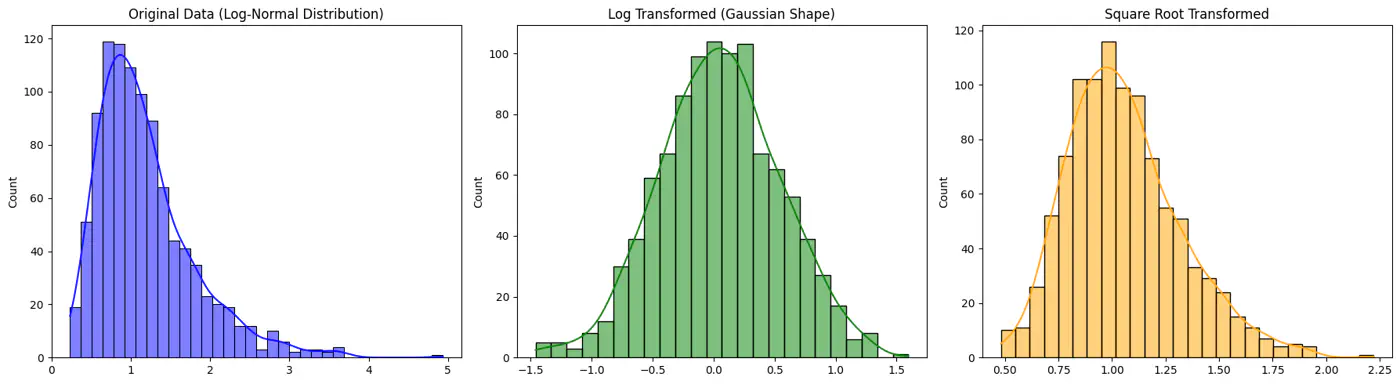
💡 If one feature ranges from 0-1 and another from 0-1000, larger feature will dominate the model.
- Standardization (Z-score) :
- μ=0, σ=1; less sensitive to outliers.
- \(x_{std} = (x − μ) / σ\)
- Min-Max Normalization:
- Maps data to specific range, typically [0,1]; sensitive to outliers.
- \(x_{minmax} = (x − min) / (max − min)\)
- Robust Scaling:
- Transforms features using median and IQR; resilient to outliers.
- \(x_{scaled}=(x-\text{median})/\text{IQR}\)
👉 Standardization Example
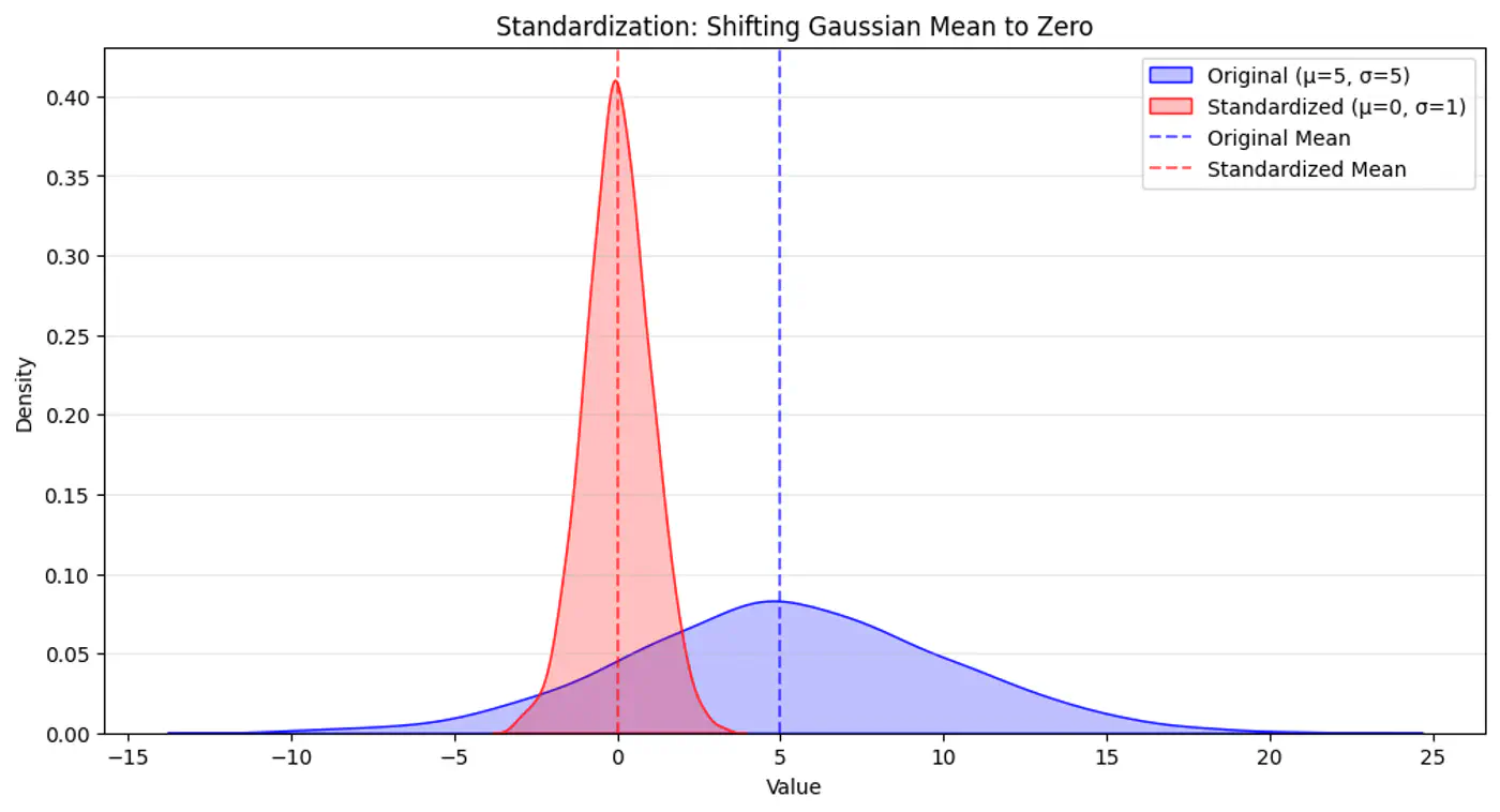
End of Section
4.2 - Categorical Variables
💡 ML models operate on numerical vectors.
👉 Categorical variables must be transformed (encoded) while preserving information and semantics.
- One Hot Encoding (OHE)
- Label Encoding
- Ordinal Encoding
- Frequency/Count Encoding
- Target Encoding
- Hash Encoding
⭐️ When the categorical data (nominal) is without any inherent ordering.
- Create binary columns per category.
- e.g.: Colors: Red, Blue, Green.
- Colors: [1,0,0], [0,1,0], [0,0,1]
Note: Use when low cardinality, or small number of unique values (<20).
⭐️ Assigns a unique integer (e.g., 0, 1, 2) to each category.
- When to use ?
- Target variable, i.e, unordered (nominal) data, in classification problems.
- e.g. encoding a city [“Paris”, “Tokyo”, “Amsterdam”] -> [1, 2, 0], (Alphabetical: Amsterdam=0, Paris=1, Tokyo=2).
- When to avoid ?
- For nominal data in linear models, because it can mislead the model to assume an order/hierarchy, when there is none.
⭐️ When categorical data has logical ordering.
Best for: Ordered (ordinal) input features.
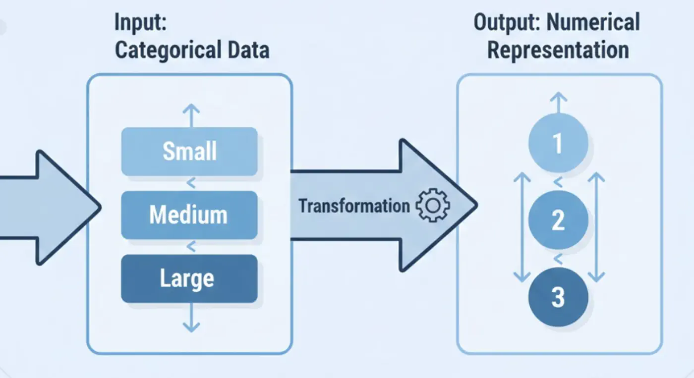
⭐️ Replace categories with their frequency or count in the dataset.
- Useful for high-cardinality features where many unique values exist.
👉 Example
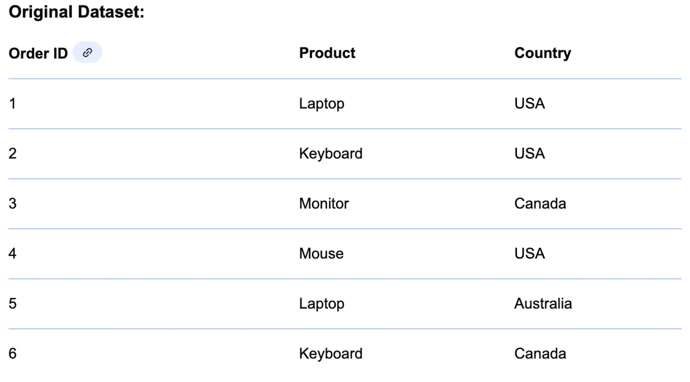
👉 Frequency of Country
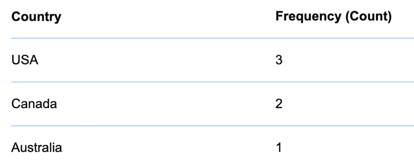
👉 Country replaced with Frequency
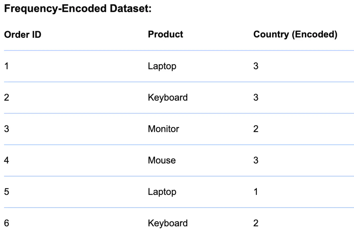
⭐️ Replace a category with the mean of the target variable for that specific category.
- When to use ?
- For high-cardinality nominal features, where one hot encoding is inefficient, e.g., zip code, product id, etc.
- Strong correlation between the category and the target variable.
- When to avoid ?
- With small datasets, because the category averages (encodings) are based on too few samples, making them unrepresentative.
- Also, it can lead to target leakage and overfitting unless proper smoothing or cross-validation techniques (like K-fold or Leave-One-Out) are used.
⭐️ Maps categories to a fixed number of features using a hash function.
Useful for high-cardinality features where we want to limit the dimensionality.
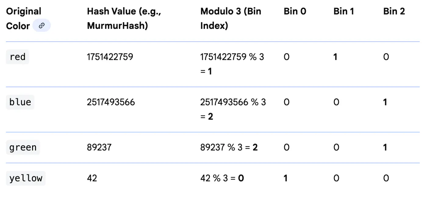
End of Section
4.3 - Feature Engineering
Create polynomial features, such as, x^2, x^3, etc., to learn non-linear relationship.
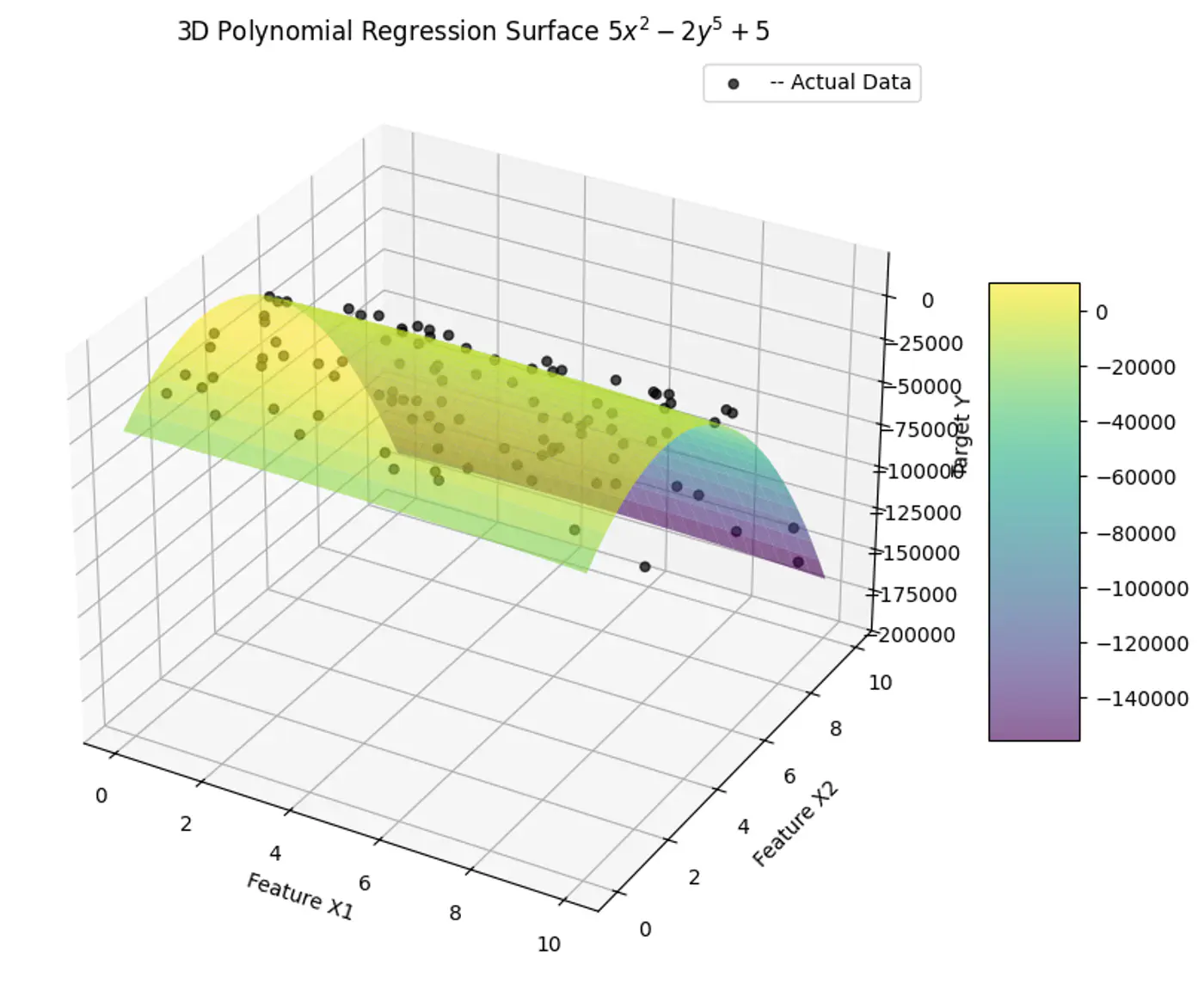
⭐️ Combine 2 or more features to capture non-linear relationship.
- e.g. combine latitude and longitude into one location feature ‘lat-long'.
⭐️ Memory-efficient 🧠 technique to convert categorical (string) data into a fixed-size numerical feature vector.
- Pros:
- Useful for high-cardinality features where we want to limit the dimensionality.
- Cons:
- Hash collisions.
- Reduced interpretability.
👉 Hash Encoding (Example)

⭐️ Group continuous numerical values into discrete categories or ‘bin’.
- e.g. divide age into groups 18-24, 25-35, 35-45, 45-55, >55 years etc.
End of Section
4.4 - Data Leakage
⭐️ Occurs when a model is trained using data that would not be available during real-world predictions,
leading to good training performance, but poor real‑world 🌎 performance.
It is essentially the model ‘cheating’ by inadvertently accessing information about the target variable.
👉Any information from the validation/test set must NOT influence training, directly or indirectly.
❓So, how do we prevent this leakage of information or data leakage from training to validation or test set ?
- ❌ Wrong: Applying preprocessing (like global StandardScaler, Mean_Imputation, Target_Encoding etc.) on the entire dataset before splitting.
- ✅ Right: Compute mean, variance, etc. only on the training data and use the same for validation and test data.
Preventing Leakage in Cross-Validation:
- ❌ Wrong: Perform preprocessing (e.g., scaling, normalization, missing value imputation) on the entire dataset before passing it to cross_val_score.
- ✅ Right: Use sklearn.pipeline.Pipeline; Pipeline ensures that the ‘validation fold’ remains unseen until the transformation is applied using the training fold’s parameters.
This happens in Time Series ⏰ data.
- ❌ Wrong: Use standard random CV; it allows the model to ‘peek into the future’.
- ✅ Right: Use Time-Series Nested Cross-Validation (Forward Chaining) instead of random shuffling.
- ❌ Wrong: Include features that are only available after the event we are trying to predict and are proxy for the target.
- e.g. Including number_of_late_payments in a model to predict whether a person applying for a bank loan will default ?
- ✅ Right: Do not include such features during training.
Group Leakage:
- ❌ Wrong: If you have multiple rows that are correlated (same user).
- For the same patient or user, you put some rows in Train and others in Test.
- ✅ Right: Use GroupKFold to ensure all data from a specific group stays together in one fold.
End of Section
4.5 - Model Interpretability
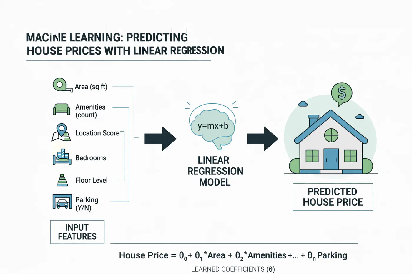
👉 Because without this capability the machine learning is like a black box to us.
👉 We should be able to answer which features had most influence on output.
⭐️ Let’s understand ‘Feature Importance’ and why the ML model output’s interpretability is important ?
Note: Weights 🏋️♀️ represent the importance of feature with standardized data.
💡 Overall model behavior + Why this prediction?
- Trust: Stakeholders must trust predictions.
- Model Debuggability: Detect leakage, spurious correlations.
- Feature engineering: Feedback loop.
- Regulatory compliance: Data privacy, GDPR.
⭐️ Stakeholders Must Trust Predictions.
- Users, executives, and clients are more likely to trust and adopt an AI system if they understand its reasoning.
- This transparency is fundamental, especially in high-stakes applications like healthcare, finance, or law, where decisions can have a significant impact.
⭐️ In many industries, regulations mandate the ability to explain decisions made by automated systems.
- For instance, the General Data Protection Regulation (GDPR) in Europe includes a “right to explanation” for individuals affected by algorithmic decisions.
- Interpretability ensures that organizations can meet these legal and ethical requirements.
End of Section
5.1 - Data Distribution Shift
- P(X | Y): Likelihood of X given Y (joint distribution)
- P(Y | X) : Model (Posterior)
- P(Y): Prior probability of the output Y.
- P(X): Evidence (marginal probability of the input X).
⭐️The input data distribution seen during training is different from the distribution seen during inference.
👉 P(X)(input) changes, but P(Y|X) (model) remains same.
- e.g. Self-driving car 🚗 trained on a bright, sunny day is used during foggy winter.
⭐️The output distribution changes, but for a given output, the input distribution remains the same.
👉 P(Y) (output) changes, but P(X|Y) remains the same.
- 😷 e.g. Flu-detection model is trained during summer, when only 1% of patients have flu.
- The same model is used during winter when 40% of patients have flu.
- 🍎 Prior probability of having flu P(Y) has changed from 1% to 40%, but the symptoms for a person to have flu P(X|Y) remains same.
⭐️ The relationship between inputs and outputs changes.
i.e the very definition of what you are trying to predict changes.
👉 Concept drifts are cyclic or seasonal.
- e.g. ‘Normal’ spending behavior in 2019 became ‘Abnormal’ during 2020 lockdowns 🔐.
End of Section
5.2 - Retraining Strategies
⭐️In a production ML environment, retraining is the ‘maintenance engine’ ⚙️ that keeps our models from becoming obsolete.
❌ Don’t ask: When do we retrain?
✅ Ask: “How do we automate the decision to retrain while balancing compute cost 💰, model risk, and data freshness?”
👉 The model is retrained on a regular schedule (e.g., daily, weekly, or monthly).
- Best for:
- Stable environments where data changes slowly.
(e.g. long-term demand forecast or a credit scoring model).
- Stable environments where data changes slowly.
- Pros:
- Highly predictable; easy to schedule compute resources; simple to implement via a cron job or Airflow DAG.
- Cons:
- Inefficient. You might retrain when not needed (wasting money 💵) or fail to retrain during a sudden market shift (losing accuracy).
👉 Retraining is initiated only when a specific performance or data metric crosses a pre-defined threshold.
- Metric Triggers:
- Performance Decay: A drop in Precision, Recall, or RMSE (requires ground-truth labels).
- Drift Detection: A high PSI (Population Stability Index) or K-S test score indicating covariate shift.
- Pros:
- Cost-effective; reacts to the ‘reality’ of the data rather than the calendar.
- Cons:
- Requires a robust monitoring stack 📺.
If the ‘trigger’ logic is buggy, the model may never update.
- Requires a robust monitoring stack 📺.
👉 Instead of retraining from scratch on a massive batch, the model is updated incrementally as new data ‘streams’ into the system.
- Mechanism: Using ‘Warm Starts’ where the model weights from the previous version are used as the starting point for the next few gradient descent steps.
- Best for:
- Recommendation engines (Netflix/TikTok) or High-Frequency Trading 💰where patterns change by the minute.
- Pros:
- Extreme ‘freshness’; low latency between data arrival and model update.
- Cons:
- High risk of ‘Catastrophic Forgetting’ (the model forgets old patterns) and high infrastructure complexity.
End of Section
5.3 - Deployment Patterns
⭐️In a production ML environment, retraining is only half the battle, we must also safely deploy the new version.
Types of deployment (most common):
- Shadow ❏ Deployment
- A/B Testing 🧪
- Canary 🦜 Deployment
👉 Safest way to deploy our model or any software update.
- Deploy the candidate model in parallel with the existing model.
- For each incoming request, route it to both models to make predictions, but only serve the existing model’s prediction to the user.
- Log the predictions from the new model for analysis purposes.
Note: When the new model’s predictions are satisfactory, we replace the existing model with the new model.
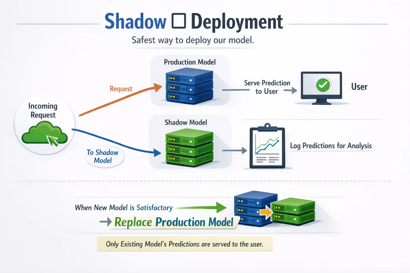
👉A/B testing is a way to compare two variants of a model.
- Deploy the candidate model in parallel with the existing model.
- A percentage of traffic🚦is routed to the candidate for predictions; the rest is routed to the existing model for predictions.
- Monitor 📺 and analyze the predictions, from both models to determine whether the difference in the two models’ performance is statistically significant.
Note: Say we run a two-sample test and get the result that model A is better than model B with the p-value of p = 0.05 or 5%.

👉 Mitigates deployment risk by incrementally shifting traffic 🚦from a model version to a new version, allowing for real-world validation on a subset of users before a full-scale rollout.
- Deploy the candidate model in parallel with the existing model.
- A percentage of traffic🚦is routed to the candidate for predictions.
- If its performance is satisfactory, increase the traffic to the candidate model.If not, abort the canary and route all the traffic🚦 back to the existing model.
- Stop when either the canary serves all the traffic🚦 (the candidate model has replaced the existing model) or when the canary is aborted.
Note: Canary releases can be used to implement A/B testing due to the similarities in their setups. However, we can do canary analysis without A/B testing.
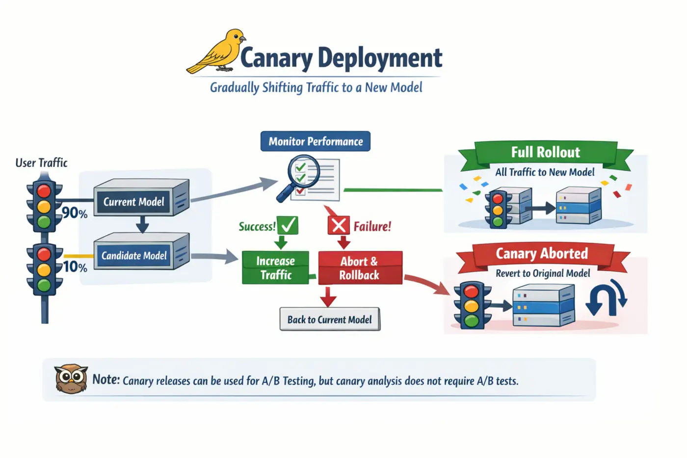
End of Section
6 - Interview Questions
Which metrics would you report and why?
We should evaluate an imbalanced classification model using metrics that that focus on performance for each class, especially the minority class.
Why ?
Say, we have a dataset with high imbalance, i.e, 99% of data belongs to positive class and only 1% of data belongs to the negative class.
In such a case, standard metrics, such as, accuracy is misleading, because a model can achieve 99% accuracy
by simply predicting positive class all the time.
So, what to do ?
First, of all, start with the confusion matrix. (focus on minority class)
It provides the raw counts of True Positives (TP), True Negatives (TN), False Positives (FP), and False Negatives (FN).
This is the foundation for all other metrics.
Confusion Matrix:
| Predicted Positive | Predicted Negative | |
|---|---|---|
| Actual Positive | True Positive (TP) | False Negative (FN) |
| Actual Negative | False Positive (FP) | True Negative (TN) |
- Precision: Of all instances the model predicted as positive, how many were actually positive?
- \( Precision = \frac{TP}{TP + FP} \)
- Use Case: The cost of a False Positive is high (e.g., marking a legitimate email as spam).
- Recall (Sensitivity): Of all actual positive instances, how many did the model find?
- \( Recall = \frac{TP}{TP + FN} \)
- Use Case: The cost of a False Negative is high (e.g., missing a cancer diagnosis or fraud transaction).
- F1-Score: Harmonic mean of precision and recall.
- \( F1 ~ Score = 2 * \frac{Precision \times Recall}{Precision + Recall}\)
- Why report F1-Score?: To balance precision and recall. A model with 1.0 precision and 0.0 recall will have an F1-score of 0.
- Precision-Recall (PR) AUC: Plots Precision against Recall for different classification thresholds.
Better than ROC curve because it uses Precision instead of False Positive Rate (FPR), which can be misleading for imbalanced data.- \(FPR = \frac{FP}{FP + TN}\)
ROC curve plots TPR vs FPR, \(FPR = \frac{FP}{FP + TN}\), so for an imbalanced data, FPR can be misleading.
So for imbalanced data, we better use Precision-Recall curve that uses Precision instead of FPR and hence is more reliable.
Let’s look at the fraud detection example below, N = 10,000 transactions, Fraud = 100, NOT fraud = 9900:
Confusion Matrix:
| Predicted Fraud | Predicted NOT Fraud | |
|---|---|---|
| Actual Fraud | 80 (TP) | 20 (FN) |
| Actual NOT Fraud | 220 (FP) | 9680 (TN) |
The FPR is very low due to the class imbalance, and hence Precision gives us a better view of the model’s performance.
👉Any information from the validation/test set must NOT influence training, directly or indirectly.
So, how do we prevent this leakage of information or data leakage from training to validation or test set ?
- Train-Test Contamination:
- ❌ Wrong: Applying preprocessing (like global StandardScaler, Mean_Imputation, Target_Encoding etc.) on the entire dataset before splitting.
- ✅ Right: Compute mean, variance, etc. only on the training data and use the same for validation and test data.
- Preventing Leakage in Cross-Validation:
- ❌ Wrong: Perform preprocessing (e.g., scaling, normalization, missing value imputation) on the entire dataset before passing it to cross_val_score.
- ✅ Right: Use sklearn.pipeline.Pipeline; Pipeline ensures that the ‘validation fold’ remains unseen until the transformation is applied using the training fold’s parameters.
- Time Series Data:
- ❌ Wrong: Use standard random CV; it allows the model to ‘peek into the future’.
- ✅ Right: Use Time-Series Nested Cross-Validation (Forward Chaining) instead of random shuffling.
- Target Leakage:
- ❌ Wrong: Include features that are only available after the event we are trying to predict and are proxy for the target.
- e.g. Including number_of_late_payments in a model to predict whether a person applying for a bank loan will default ?
- ✅ Right: Do not include such features during training.
- Group Leakage:
- ❌ Wrong: If you have multiple rows that are correlated (same user).
- For the same patient or user, you put some rows in Train and others in Test.
- ✅ Right: Use GroupKFold to ensure all data from a specific group stays together in one fold.
Bias-Variance Decomposition:
For Mean Squared Error (MSE) = \(\frac{1}{n} \sum_{i=1}^n (y_i - \hat{y_i})^2\)
Total Error = Bias^2 + Variance + Irreducible Error
- Bias = Systematic Error
- Bias measures how far the average prediction of a model is from the true value.
- Variance = Sensitivity to Data
- Variance measures how much the predictions of a model vary for different training datasets.
- Irreducible Error = Sensor noise, Human randomness
- Inherent uncertainty in the data generation process itself and cannot be reduced by any model.
Bias-Variance Trade-Off:
- High Bias (Underfitting): A model with high bias is too simple to capture the underlying patterns in the data
- e.g., fitting a straight line to curved data.
- High Variance (Overfitting): A model with high variance is too complex and learns the noise in the training data rather than the true relationship
- e.g., a high-degree polynomial curve that perfectly fits training data points but performs poorly on new data.
🎯 The goal is to find a balance; a ‘sweet spot’ that minimizes the total error.
🦉 A good model ‘generalizes’ well, i.e., neither too simple (low bias) nor too complex (low variance).
- L1 Regularization:
- \( \underset{w}{\mathrm{min}}\ J_{reg}(w) = \underset{w}{\mathrm{min}}\ J(w) + \lambda_1.\sum_{j=1}^n |w_j| \)
- L2 Regularization:
- \( \underset{w}{\mathrm{min}}\ J_{reg}(w) = \underset{w}{\mathrm{min}}\ J(w) + \lambda_2.\sum_{j=1}^n w_j^2 \)
L1 regularization produces sparse solutions when regularization coefficient \(\lambda_1\) is high.
- Because the gradient of L1 penalty (absolute function) is a constant value, i.e, \(\pm 1\), this means a constant reduction in weight at each step, making it gradually reach to 0 in finite steps.
- Whereas, the derivative of L2 penalty is proportional to the weight (\(2w_j\)) and as the weight reaches close to 0, the gradient also becomes very small, this means that the weight will become very close to 0, but not exactly equal to 0.
💡 Heteroscedasticity = Variance NOT Constant
Note: Linear regression assumes that the data has homoscedasticity (constant variance).
Ordinary Least Squares (OLS) is an unweighted estimator. It treats every data point as equally ‘informative’.
- Under Homoscedasticity: Every point has the same amount of noise, so giving them equal weight is logical.
- Under Heteroscedasticity: Some points have very low variance (high certainty) and some have very high variance (lots of noise).
👉 By treating all the points equally, OLS is ‘wasting’ the precision of the low-variance points and being ‘skewed’ by the high-variance points.
This is why OLS is no longer efficient; does not produce the smallest possible standard errors.
Which means:
- t-tests become unreliable.
- p-values become misleading.
- Confidence intervals are wrong.
👉 OLS is NO longer B.L.U.E. (Best Linear Unbiased Estimator).
- While the coefficients remain unbiased,
they are no longer the ‘best’ because there is another estimator (like Weighted Least Squares) that could provide a lower variance.
👉 How to Test for Heteroscedasticity ?
- Visual (Residual Plot):
- Heteroscedasticity: The points form a ‘fan’ or ‘funnel’ shape, widening or narrowing as values increase.
- Homoscedasticity: The points look like a random ‘cloud’ with consistent thickness.
- Breusch–Pagan Test
- White Test
- Goldfeld–Quandt Test
Probability vs. Likelihood:
Difference lies in which variable is fixed and which is varying.
- Probability(Forward View):
- Quantifies the chance of observing a specific outcome given a known, fixed parameters \(\theta\).
- Likelihood(Backward/Inverse View):
- Inverse concept used for inference (working backward from results to causes).
- It is a function of the parameters \(\theta\) and measures how ‘likely’ a specific set of parameters makes the observed (fixed) data appear.
MLE vs. MAP:
Both help us answer the question:
Which parameter \(\theta\) best explains the data we just saw?
- Maximum Likelihood Estimation (MLE):
- MLE believes the data should speak for itself.
- It asks: ‘Which value of \(\theta\) makes the observed data most probable?’
- It ignores any outside context or common sense.
- Maximum A Posteriori (MAP):
- MAP believes the data is important, but so is prior knowledge.
- It asks: ‘Given the data AND what we already know about the problem at hand, which value of \(\theta\) is most likely?’
The relationship between them is rooted in Bayes’ Theorem:
\[P(\theta \mid \text{data}) = \frac{P(\text{data} \mid \theta) P(\theta)}{P(\text{data})}\]- MLE maximizes only the Likelihood: \(P(\text{data} \mid \theta)\)
- MAP maximizes the Posterior: \(P(\text{data} \mid \theta) P(\theta)\)
Note:
- P(data) is a constant (a ’normalizing factor’), so we ignore it during maximization.
- For a prior with uniform distribution where every value is equally likely, MAP becomes MLE.
👉 Coin Toss Example:
- Data: Toss the coin 3 times, 2H + 1T.
- MLE: Probability of heads (\(\theta\))
- \(\theta_{MLE}\) = 2/3 = 0.67
- MAP (with prior belief that coin is fair)
- Assume prior: \(\theta \sim \beta(10,10)\)
- Posterior = \(\beta(12,11)\)
- \(\theta_{MAP}\) = 0.52 (Prior pulls estimate towards 0.5)
- MLE: Probability of heads (\(\theta\))
✅ Use MLE when:
- large dataset.
- no reliable prior knowledge.
✅ Use MAP when:
- small dataset.
- reliable prior/domain knowledge.
Entropy (H) is a measure of impurity or randomness in a dataset.
For binary classification, where the outcome is Yes/No, 0/1 etc., entropy will be:
\[H(S) = -p \log_2(p) - (1-p) \log_2(1-p)\]- Max Entropy: H(S) = 1, when the classes are split 50/50 (maximum uncertainty).
- Min Entropy: H(S) = 0 when the set is pure (all examples belong to one class).
Information Gain:
️Measures the reduction in entropy (uncertainty) achieved by splitting a dataset based on a specific attribute.
Note: The goal of a decision tree algorithm is to find the split that maximizes information gain, meaning it removes the most uncertainty from the data.
👉 To understand how a Decision Tree selects the ‘best’ root node, let’s use the example below:
The Dataset: “Will they buy the product?”
| ID | Age | Income | Credit Score | Buy? (Target) |
|---|---|---|---|---|
| 1 | Youth | High | Good | No |
| 2 | Youth | High | Excellent | No |
| 3 | Middle | High | Good | Yes |
| 4 | Senior | Medium | Good | Yes |
| 5 | Senior | Low | Good | Yes |
| 6 | Senior | Low | Excellent | No |
- Calculate parent node’s entropy:
- P(yes) = P(no) = 3/6 = 0.5
- \(H(Parent) = -(0.5 \log_2 0.5 + 0.5 \log_2 0.5) = \mathbf{1.0}\)
- Evaluate feature ‘Age’:
- Youth: 2 samples (0 Yes, 2 No). \(H(Youth) = \mathbf{0}\)
- Middle: 1 sample (1 Yes, 0 No). \(H(Middle) = \mathbf{0}\)
- Senior: 3 samples (2 Yes, 1 No). \(H(Senior) = -(\frac{2}{3} \log_2 \frac{2}{3} + \frac{1}{3} \log_2 \frac{1}{3}) \approx \mathbf{0.918}\)
- Weighted Entropy for Age:
- \((\frac{2}{6} \times 0) + (\frac{1}{6} \times 0) + (\frac{3}{6} \times 0.918) = \mathbf{0.459}\)
- Information Gain (Age): \(1.0 - 0.459 = \mathbf{0.541}\)
- Evaluate feature ‘Income’:
- High: 3 samples (1 Yes, 2 No). \(H(High) \approx \mathbf{0.918}\)
- Medium: 1 sample (1 Yes, 0 No). \(H(Medium) = \mathbf{0}\)
- Low: 2 samples (1 Yes, 1 No). \(H(Low) = \mathbf{1.0}\)
- Weighted Entropy for Income:
- \((\frac{3}{6} \times 0.918) + (\frac{1}{6} \times 0) + (\frac{2}{6} \times 1.0) = \mathbf{0.792}\)
- Information Gain (Income): \(1.0 - 0.792 = \mathbf{0.208}\)
- Evaluate feature ‘Credit Score’
- Good: 4 samples (3 Yes, 1 No). \(H(Good) \approx \mathbf{0.811}\)
- Excellent: 2 samples (0 Yes, 2 No). \(H(Excellent) = \mathbf{0}\)
- Weighted Entropy for Credit Score:
- \((\frac{4}{6} \times 0.811) + (\frac{2}{6} \times 0) = \mathbf{0.541}\)
- Information Gain (Credit Score): \(1.0 - 0.541 = \mathbf{0.459}\)
- The Decision Tree algorithm compares the information gain for all the features, and splits on the feature with maximum information gain.
- Here in our case it is “Age”, IG = 0.541.
- The algorithm chooses ‘Age’ as the root node.
- Splits the data into three branches (Youth, Middle, Senior).
End of Section