Messy and Incomplete.
We need to pre-process the data to make it:

• Clean
• Consistent
• Mathematically valid
• Computationally stable

👉 So that, the machine learning algorithm can safely consume the data.

• Missing Completely At Random (MCAR)
  • The missingness occurs entirely by chance, such as due to a technical glitch during data collection or a random human error in data entry.
• Missing At Random (MAR)
  • The probability of missingness depends on the observed data and not on the missing value itself.
  • e.g. In some survey, the age of many females are missing, because they may not like to disclose the information.
• Missing Not At Random (MNAR)
  • The probability of missingness is directly related to the unobserved missing value itself.
  • e.g. Individuals with very high incomes 💰may intentionally refuse to report their salary due to privacy concerns, making the missing data directly dependent on the high income 💰value itself.

• Simple Imputation:
  • Mean: Normally distributed numerical features.
  • Median: Skewed numerical features.
  • Mode: Categorical features, most frequent.
• KNN Imputation:
  • Replace the missing value with mean/median/mode of ‘k’ nearest (similar) neighbors of the missing value.
• Predictive Imputation:
  • Use another ML model to estimate missing values.
• Multivariate Imputation by Chained Equations (MICE):
  • Iteratively models each variable with missing values as a function of other variables using flexible regression models (linear regression, logistic regression, etc.) in a ‘chained’ or sequential process.
  • Creates multiple datasets, using slightly different random starting points.

🦄 Outliers are extreme or unusual data points, can mislead models, causing inaccurate predictions.

• Remove invalid or corrupted data.
• Replace (Impute): Median or capped value to reduce impact.
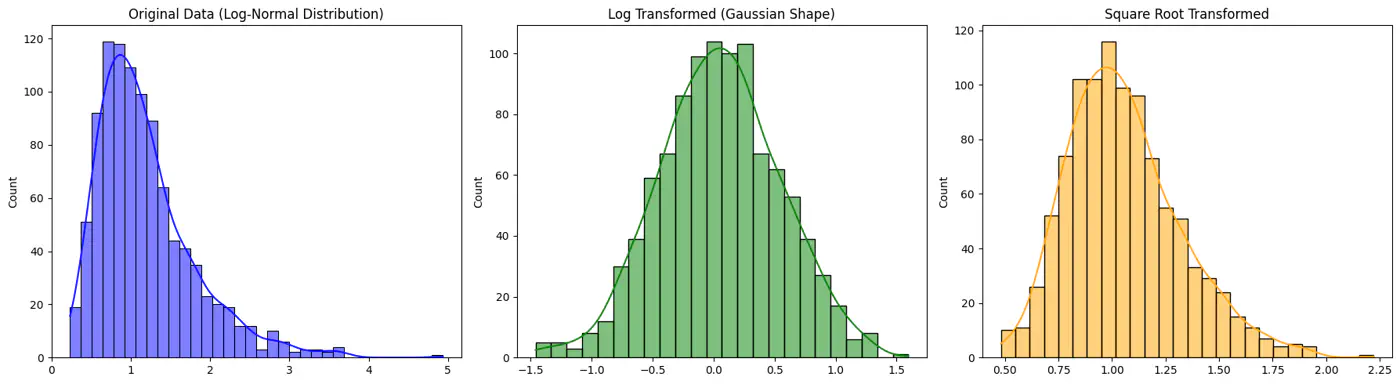
• Transform: Apply log or square root to reduce skew.

👉 For example: Log and Square Root Transformed Data

💡 If one feature ranges from 0-1 and another from 0-1000, larger feature will dominate the model.

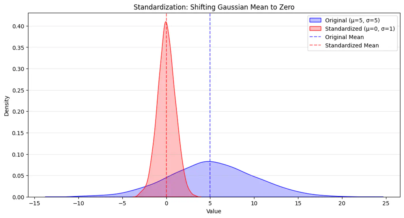
• Standardization (Z-score) :
  • μ=0, σ=1; less sensitive to outliers.
  • \(x_{std} = (x − μ) / σ\)
• Min-Max Normalization:
  • Maps data to specific range, typically [0,1]; sensitive to outliers.
  • \(x_{minmax} = (x − min) / (max − min)\)
• Robust Scaling:
  • Transforms features using median and IQR; resilient to outliers.
  • \(x_{scaled}=(x-\text{median})/\text{IQR}\)

👉 Standardization Example

💡 ML models operate on numerical vectors.

👉 Categorical variables must be transformed (encoded) while preserving information and semantics.

• One Hot Encoding (OHE)
• Label Encoding
• Ordinal Encoding
• Frequency/Count Encoding
• Target Encoding
• Hash Encoding

⭐️ When the categorical data (nominal) is without any inherent ordering.

• Create binary columns per category.
  • e.g.: Colors: Red, Blue, Green.
  • Colors: [1,0,0], [0,1,0], [0,0,1]

Note: Use when low cardinality, or small number of unique values (<20).

⭐️ Assigns a unique integer (e.g., 0, 1, 2) to each category.

• When to use ?
  • Target variable, i.e, unordered (nominal) data, in classification problems.
  • e.g. encoding a city [“Paris”, “Tokyo”, “Amsterdam”] -> [1, 2, 0], (Alphabetical: Amsterdam=0, Paris=1, Tokyo=2).
• When to avoid ?
  • For nominal data in linear models, because it can mislead the model to assume an order/hierarchy, when there is none.

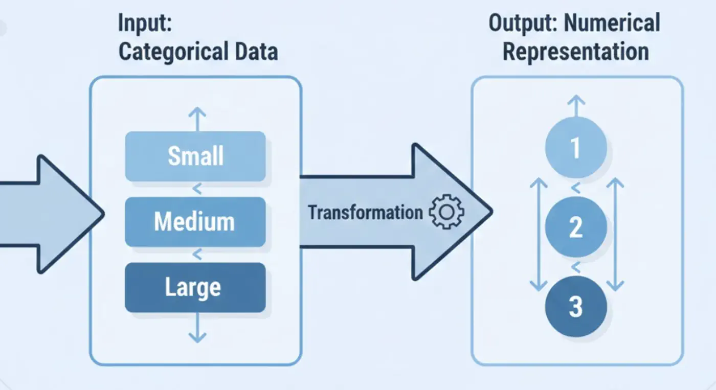
⭐️ When categorical data has logical ordering.

• Best for: Ordered (ordinal) input features.

  

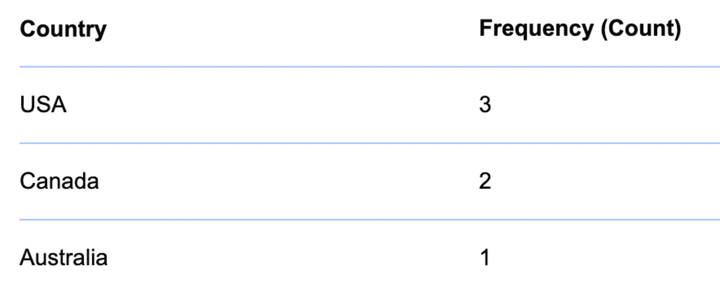
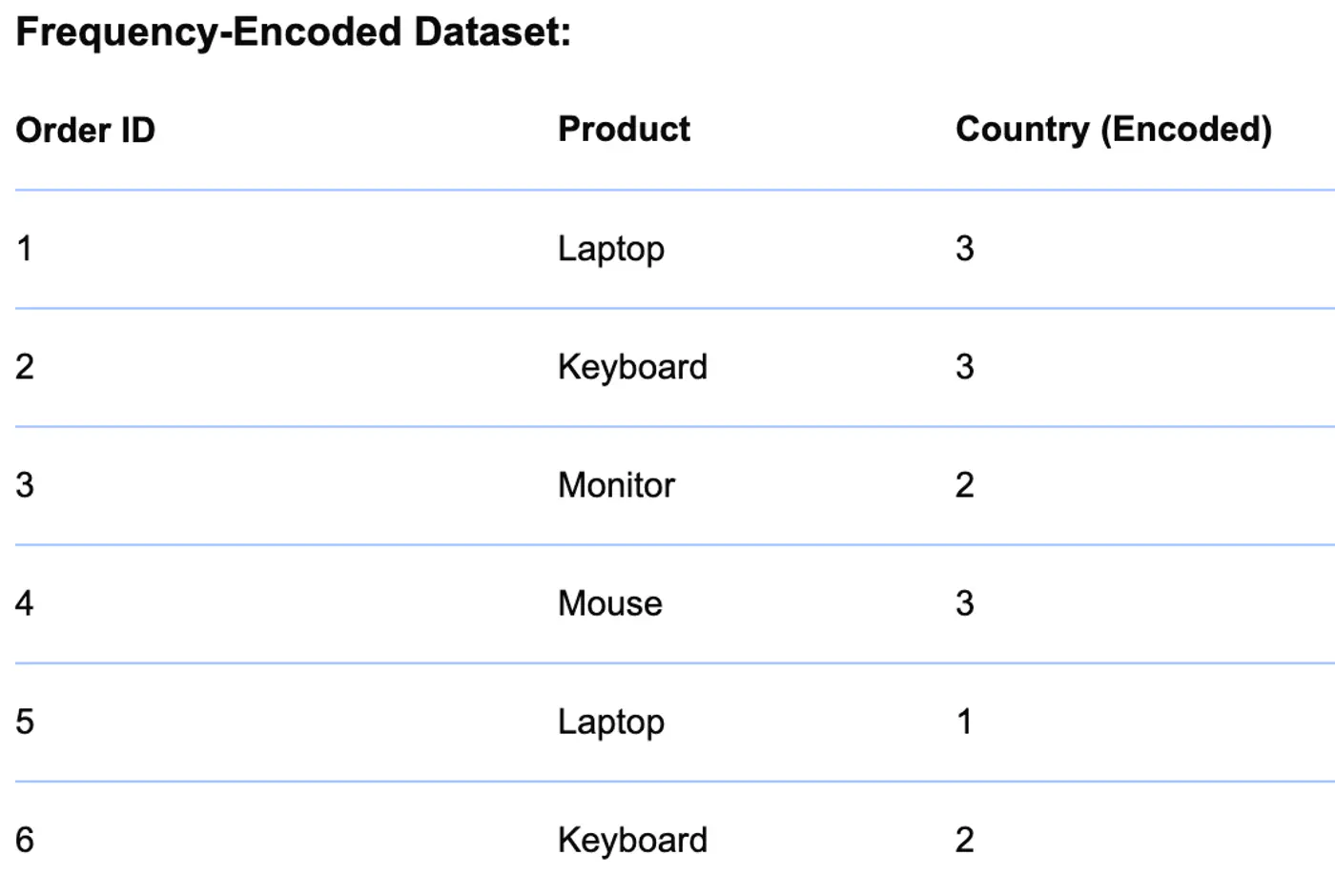
⭐️ Replace categories with their frequency or count in the dataset.

• Useful for high-cardinality features where many unique values exist.

👉 Example

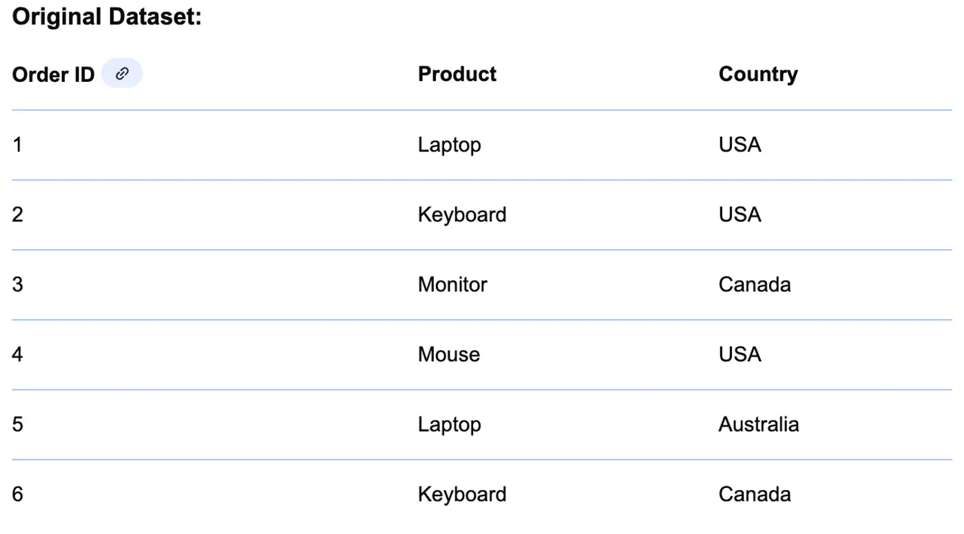
👉 Frequency of Country

👉 Country replaced with Frequency

⭐️ Replace a category with the mean of the target variable for that specific category.

• When to use ?
  • For high-cardinality nominal features, where one hot encoding is inefficient, e.g., zip code, product id, etc.
  • Strong correlation between the category and the target variable.
• When to avoid ?
  • With small datasets, because the category averages (encodings) are based on too few samples, making them unrepresentative.
  • Also, it can lead to target leakage and overfitting unless proper smoothing or cross-validation techniques (like K-fold or Leave-One-Out) are used.

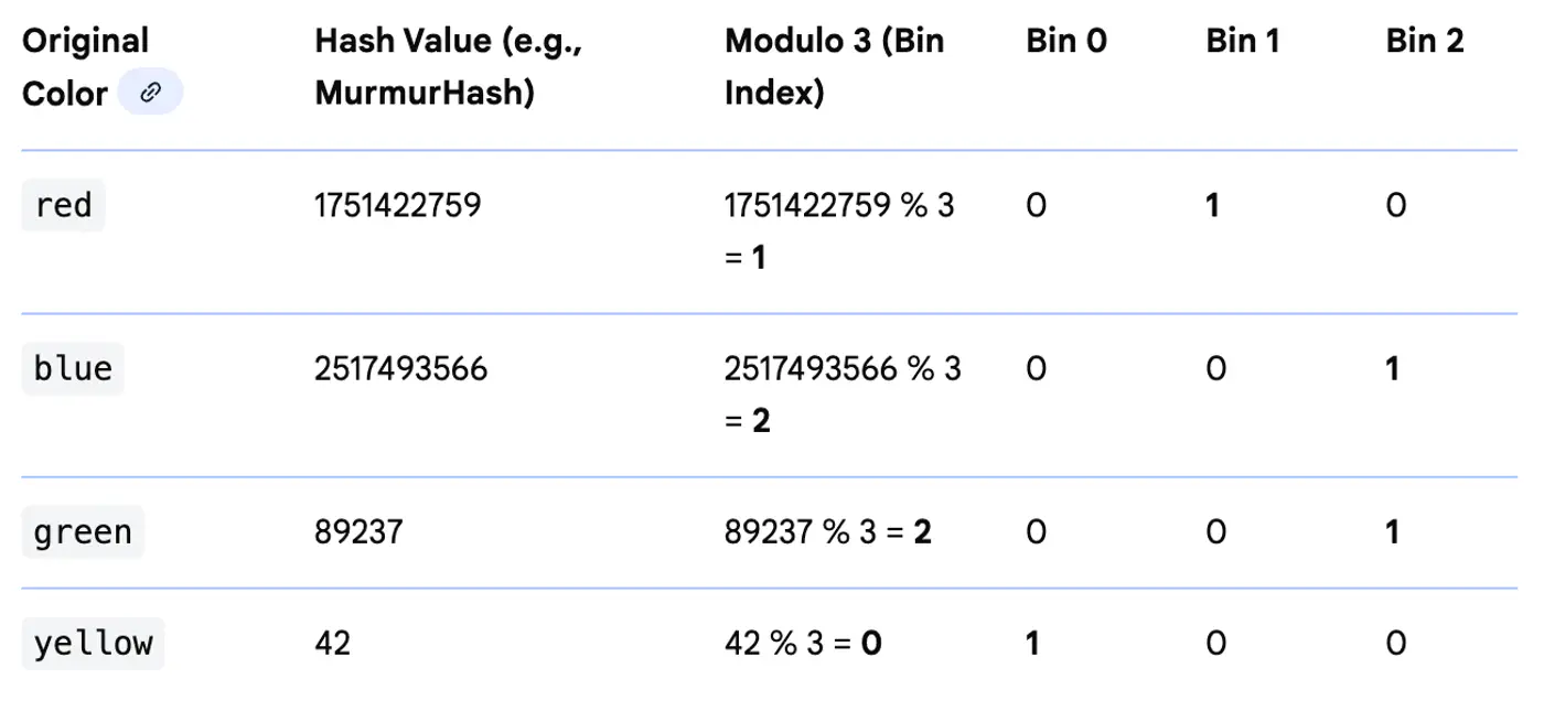
⭐️ Maps categories to a fixed number of features using a hash function.

• Useful for high-cardinality features where we want to limit the dimensionality.

  

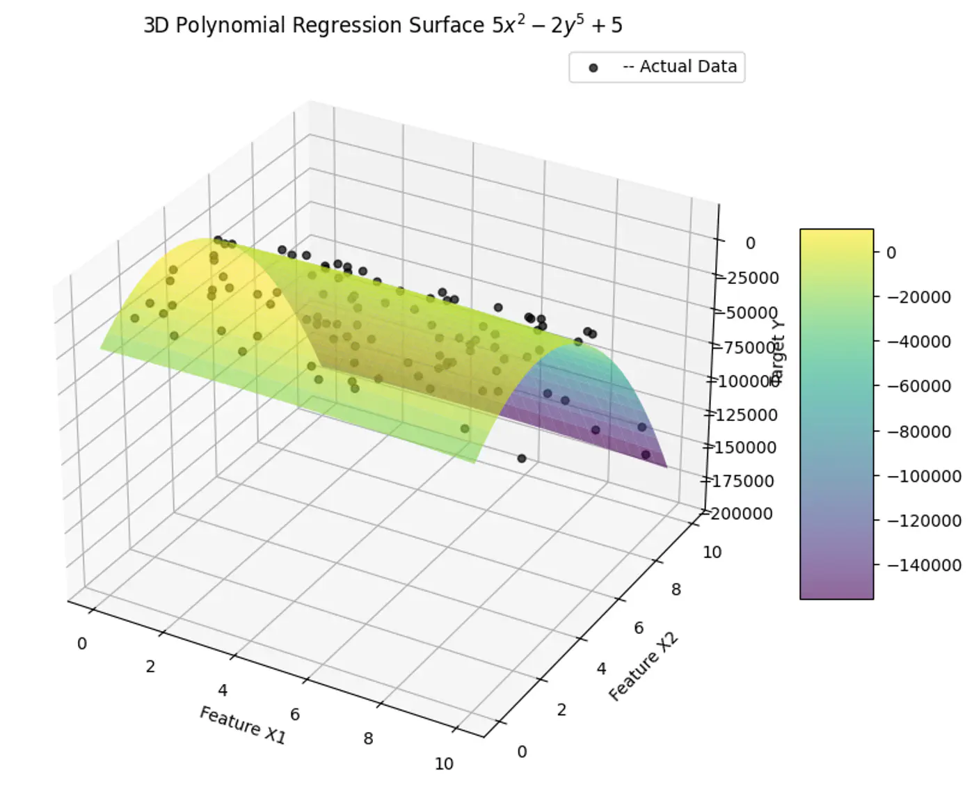
Create polynomial features, such as, x^2, x^3, etc., to learn non-linear relationship.

⭐️ Combine 2 or more features to capture non-linear relationship.

• e.g. combine latitude and longitude into one location feature ‘lat-long'.

⭐️ Memory-efficient 🧠 technique to convert categorical (string) data into a fixed-size numerical feature vector.

• Pros:
  • Useful for high-cardinality features where we want to limit the dimensionality.
• Cons:
  • Hash collisions.
  • Reduced interpretability.

👉 Hash Encoding (Example)

⭐️ Group continuous numerical values into discrete categories or ‘bin’.

• e.g. divide age into groups 18-24, 25-35, 35-45, 45-55, >55 years etc.

⭐️ Including features that are only available after the event we are trying to predict.

• e.g. Including number_of_late_payments in a model to predict whether a person applying for a bank loan 💵 will default ?

⭐️ Using future data to predict the past.

• Fix: Use Time-Series ⏰ Cross-Validation (Walk-forward validation) instead of random shuffling.

⭐️ Applying preprocessing (like global StandardScaler or Mean_Imputation) on the entire dataset before splitting.

• Fix: Compute mean, variance, etc. only on the training 🏃‍♂️data and use the same for validation and test data.

👉 Because without this capability the machine learning is like a black box to us.

👉 We should be able to answer which features had most influence on output.

⭐️ Let’s understand ‘Feature Importance’ and why the ML model output’s interpretability is important ?

Note: Weights 🏋️‍♀️ represent the importance of feature with standardized data.

💡 Overall model behavior + Why this prediction?

• Trust: Stakeholders must trust predictions.
• Model Debuggability: Detect leakage, spurious correlations.
• Feature engineering: Feedback loop.
• Regulatory compliance: Data privacy, GDPR.

⭐️ Stakeholders Must Trust Predictions.

• Users, executives, and clients are more likely to trust and adopt an AI system if they understand its reasoning.
• This transparency is fundamental, especially in high-stakes applications like healthcare, finance, or law, where decisions can have a significant impact.

⭐️ In many industries, regulations mandate the ability to explain decisions made by automated systems.

• For instance, the General Data Protection Regulation (GDPR) in Europe includes a “right to explanation” for individuals affected by algorithmic decisions.
• Interpretability ensures that organizations can meet these legal and ethical requirements.