This is the multi-page printable view of this section. Click here to print.
ML System
1 - Data Distribution Shift
- P(X | Y): Likelihood of X given Y (joint distribution)
- P(Y | X) : Model (Posterior)
- P(Y): Prior probability of the output Y.
- P(X): Evidence (marginal probability of the input X).
The input data distribution seen during training is different from the distribution seen during inference.
P(X)(input) changes, but P(Y|X) (model) remains same.
- e.g. Self-driving car trained on a bright, sunny day is used during foggy winter.
The output distribution changes, but for a given output, the input distribution remains the same.
P(Y) (output) changes, but P(X|Y) remains the same.
- e.g. Flu-detection model is trained during summer, when only 1% of patients have flu.
- The same model is used during winter when 40% of patients have flu.
- Prior probability of having flu P(Y) has changed from 1% to 40%, but the symptoms for a person to have flu P(X|Y) remains same.
The relationship between inputs and outputs changes.
i.e, the very definition of what you are trying to predict changes.
Concept drifts are cyclic or seasonal.
- e.g. ‘Normal’ spending behavior in 2019 became ‘Abnormal’ during 2020 lockdowns .
2 - Retraining Strategies
In a production ML environment, retraining is the ‘maintenance engine’ ️ that keeps our models from becoming obsolete.
❌ Don’t ask: When do we retrain?
✅ Ask: “How do we automate the decision to retrain while balancing compute cost , model risk, and data freshness?”
The model is retrained on a regular schedule (e.g., daily, weekly, or monthly).
- Best for:
- Stable environments where data changes slowly.
(e.g. long-term demand forecast or a credit scoring model).
- Stable environments where data changes slowly.
- Pros:
- Highly predictable; easy to schedule compute resources; simple to implement via a cron job or Airflow DAG.
- Cons:
- Inefficient. You might retrain when not needed (wasting money ) or fail to retrain during a sudden market shift (losing accuracy).
Retraining is initiated only when a specific performance or data metric crosses a pre-defined threshold.
- Metric Triggers:
- Performance Decay: A drop in Precision, Recall, or RMSE (requires ground-truth labels).
- Drift Detection: A high PSI (Population Stability Index) or K-S test score indicating covariate shift.
- Pros:
- Cost-effective; reacts to the ‘reality’ of the data rather than the calendar.
- Cons:
- Requires a robust monitoring stack .
If the ‘trigger’ logic is buggy, the model may never update.
- Requires a robust monitoring stack .
Instead of retraining from scratch on a massive batch, the model is updated incrementally as new data ‘streams’ into the system.
- Mechanism: Using ‘Warm Starts’ where the model weights from the previous version are used as the starting point for the next few gradient descent steps.
- Best for:
- Recommendation engines (Netflix/TikTok) or High-Frequency Trading where patterns change by the minute.
- Pros:
- Extreme ‘freshness’; low latency between data arrival and model update.
- Cons:
- High risk of ‘Catastrophic Forgetting’ (the model forgets old patterns) and high infrastructure complexity.
3 - Deployment Patterns
In a production ML environment, retraining is only half the battle, we must also safely deploy the new version.
Types of deployment (most common):
- Shadow Deployment
- A/B Testing - Canary Deployment
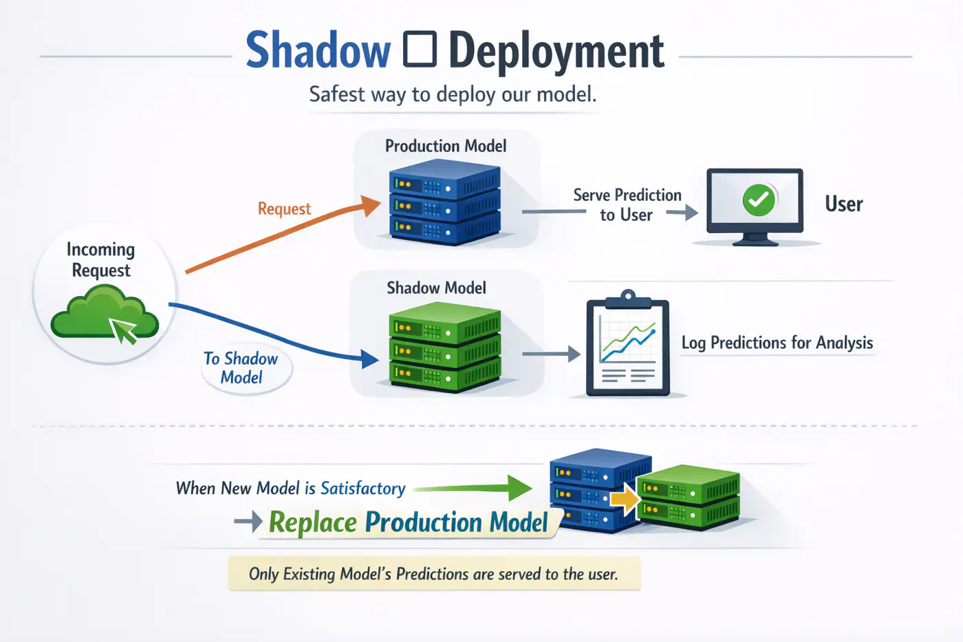
Safest way to deploy our model or any software update.
- Deploy the candidate model in parallel with the existing model.
- For each incoming request, route it to both models to make predictions, but only serve the existing model’s prediction to the user.
- Log the predictions from the new model for analysis purposes.
Note: When the new model’s predictions are satisfactory, we replace the existing model with the new model.
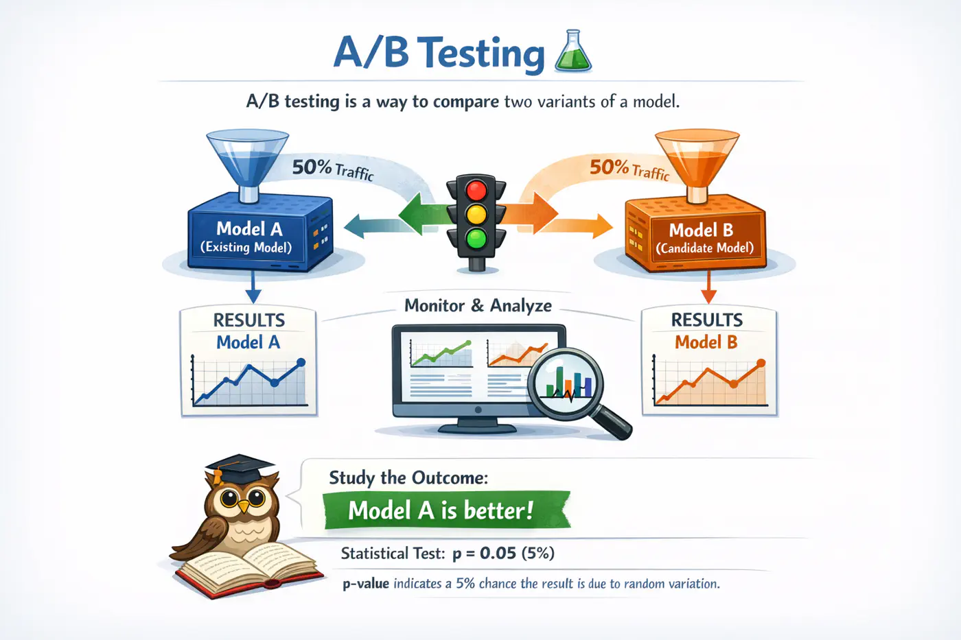
A/B testing is a way to compare two variants of a model.
- Deploy the candidate model in parallel with the existing model.
- A percentage of trafficis routed to the candidate for predictions; the rest is routed to the existing model for predictions.
- Monitor and analyze the predictions, from both models to determine whether the difference in the two models’ performance is statistically significant.
Note: Say we run a two-sample test and get the result that model A is better than model B with the p-value of p = 0.05 or 5%.
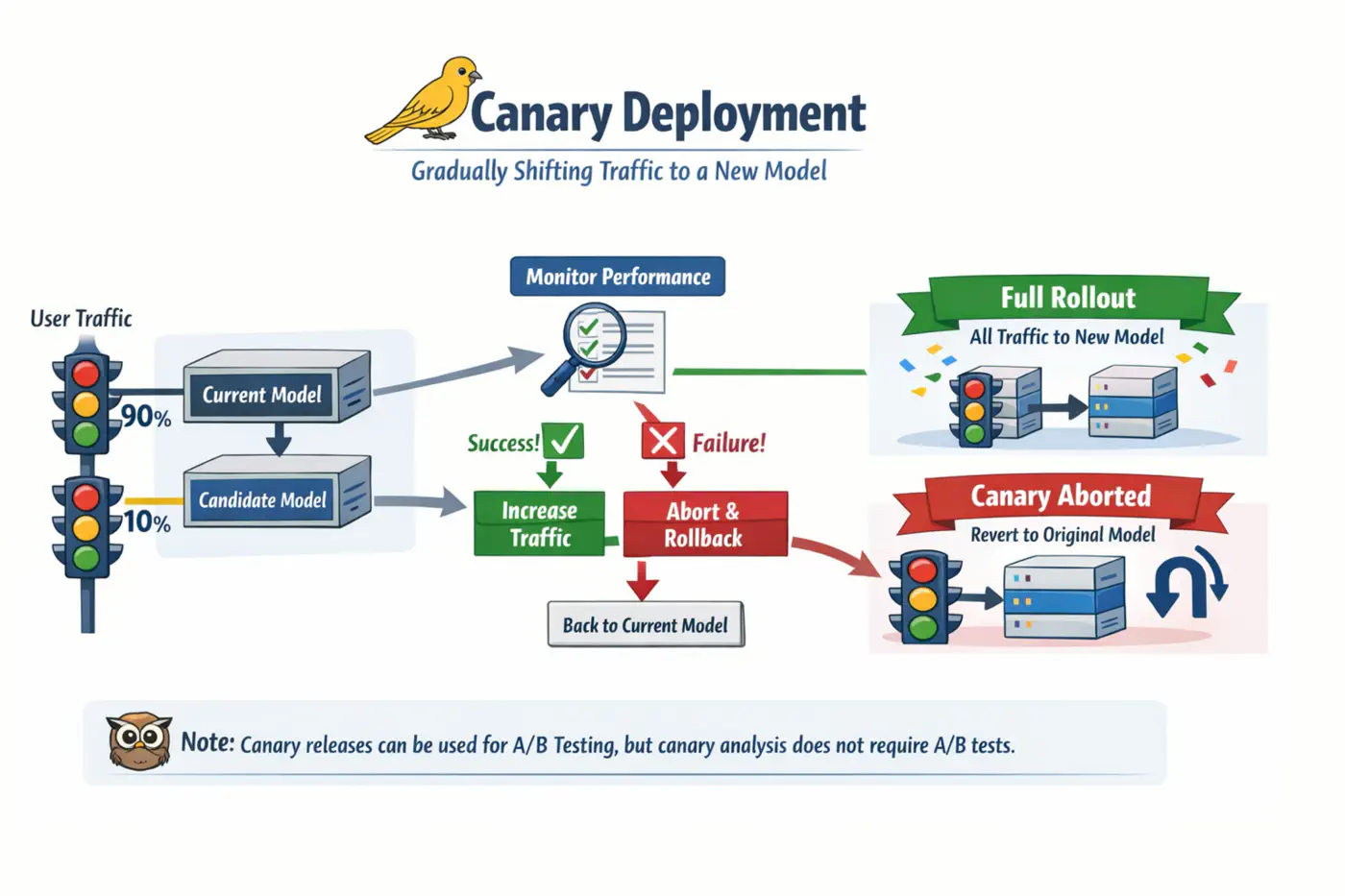
Mitigates deployment risk by incrementally shifting traffic from a model version to a new version, allowing for real-world validation on a subset of users before a full-scale rollout.
- Deploy the candidate model in parallel with the existing model.
- A percentage of trafficis routed to the candidate for predictions.
- If its performance is satisfactory, increase the traffic to the candidate model.If not, abort the canary and route all the trafficback to the existing model.
- Stop when either the canary serves all the traffic(the candidate model has replaced the existing model) or when the canary is aborted.
Note: Canary releases can be used to implement A/B testing due to the similarities in their setups. However, we can do canary analysis without A/B testing.