This is the multi-page printable view of this section. Click here to print.
Supervised Learning
- 1: Linear Regression
- 1.1: Meaning of 'Linear'
- 1.2: Meaning of 'Regression'
- 1.3: Linear Regression
- 1.4: Probabilistic Interpretation
- 1.5: Convex Function
- 1.6: Gradient Descent
- 1.7: Polynomial Regression
- 1.8: Data Splitting
- 1.9: Cross Validation
- 1.10: Bias Variance Tradeoff
- 1.11: Regularization
- 1.12: Regression Metrics
- 1.13: Assumptions
- 2: Logistic Regression
- 2.1: Binary Classification
- 2.2: Log Loss
- 2.3: Regularization
- 2.4: Log Odds
- 2.5: Probabilistic Interpretation
- 3: K Nearest Neighbors
- 3.1: KNN Introduction
- 3.2: KNN Optimizations
- 3.3: Curse Of Dimensionality
- 3.4: Bias Variance Tradeoff
- 4: Decision Tree
- 4.1: Decision Trees Introduction
- 4.2: Purity Metrics
- 4.3: Decision Trees For Regression
- 4.4: Regularization
- 4.5: Bagging
- 4.6: Random Forest
- 4.7: Extra Trees
- 4.8: Boosting
- 4.9: AdaBoost
- 4.10: Gradient Boosting Machine
- 4.11: GBDT Algorithm
- 4.12: GBDT Example
- 4.13: Advanced GBDT Algorithms
- 4.14: XgBoost
- 4.15: LightGBM
- 4.16: CatBoost
- 5: Support Vector Machine
- 5.1: SVM Intro
- 5.2: Hard Margin SVM
- 5.3: Soft Margin SVM
- 5.4: Primal Dual Equivalence
- 5.5: Kernel Trick
- 5.6: RBF Kernel
- 5.7: Support Vector Regression
- 6: Naive Bayes'
- 6.1: Naive Bayes Intro
- 6.2: Naive Bayes Issues
- 6.3: Naive Bayes Example
1.1 - Meaning of 'Linear'
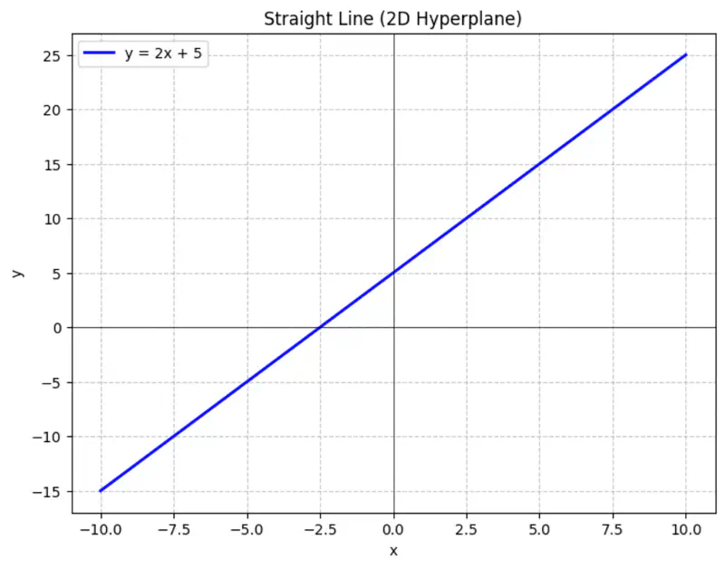
Equation of a line is of the form \(y = mx + c\).
To represent a line in 2D space, we need 2 things:
- m = slope or direction of the line
- c = y-intercept or distance from the origin
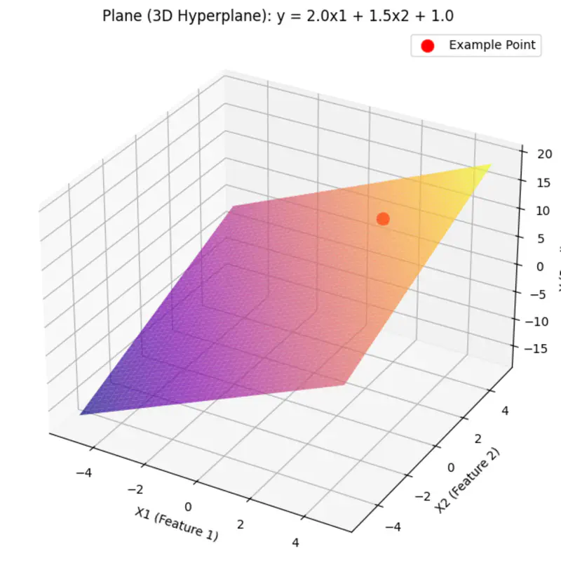
Similarly,
A hyperplane is a lower (d-1) dimensional sub-space that divides a d-dimensional space into 2 distinct parts.
Equation of a hyperplane:
Here, ‘y’ is expressed as a linear combination of parameters - \( w_0, w_1, w_2, \dots, w_n \)
Hence - Linear means the model is ‘linear’ with respect to its parameters NOT the variables.
Read more about Hyperplane
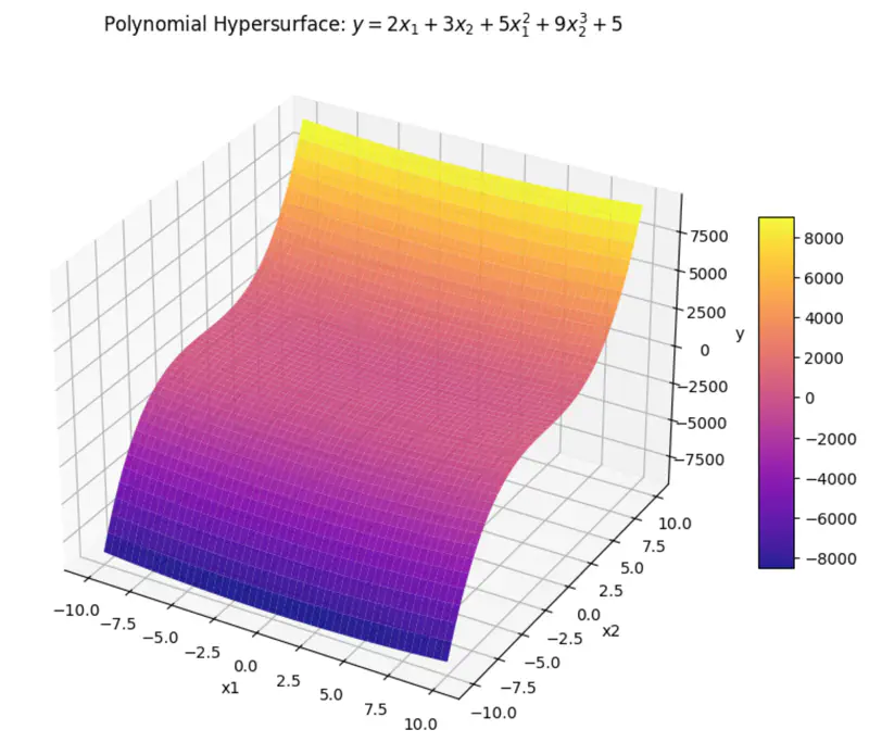
can be rewritten as:
\[y = w_1x_1 + w_2x_2 + w_3x_3 + w_4x_4 + w_0\]where, \(x_3 = x_1^2 ~ and ~ x_4 = x_2^3 \)
\(x_3 ~ and ~ x_4 \) are just 2 new (polynomial) variables.
And, ‘y’ is still a linear combination of parameters: \(w_0, w_1, \dots w_4\)
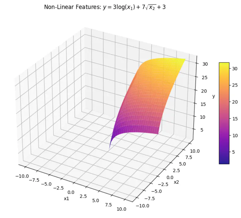
can be rewritten as:
\[y = w_1x_1 + w_2x_2 + w_0\]where, \(x_1 = log(x) ~ and ~ x_2 = \sqrt{x} \)
\(x_1 ~ and ~ x_2 \) are are transformations of variable \(x\).
And, ‘y’ is still a linear combination of parameters: \(w_0, w_1, ~and~ w_2\)
Even if we take log, we get:
\[log(y) = w_1log(x_1) + w_2log(x_2) + log(w_0)\]here, \(log(w_0) \) parameter is NOT linear.
End of Section
1.2 - Meaning of 'Regression'
Regression = Going Back
Regression has a very specific historical origin that is different from its current statistical meaning.
Sir Francis Galton (19th century), cousin of Charles Darwin, coined 🪙 this term.
Observation:
Galton observed that -
the children 👶 of unusually tall ⬆️ parents 🧑🧑🧒🧒,
tended to be shorter ⬇️ than their parents 🧑🧑🧒🧒,
and children 👶 of unusually short ⬇️ parents 🧑🧑🧒🧒,
tended to be taller ⬆️ than their parents 🧑🧑🧒🧒.
Galton named this biological tendency - ‘regression towards mediocrity/mean’.
Galton used method of least squares to model this relationship, by fitting a line to the data 📊.
Regression = Fitting a Line
Over time ⏳, the name ‘regression’ got permanently attached to the method of fitting line to the data 📊.
Today in statistics and machine learning, ‘regression’ universally refers to the method of finding the
‘line of best fit’ for a set of data points, NOT the concept of ‘regressing towards the mean’.
End of Section
1.3 - Linear Regression
Let’s understand linear regression using an example to predict salary.
Predict the salary 💰 of an IT employee, based on various factors, such as, years of experience, domain, role, etc.
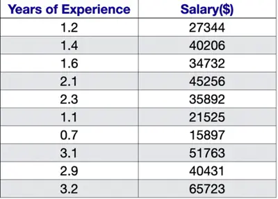
Let’s start with a simple problem and predict the salary using only one input feature.
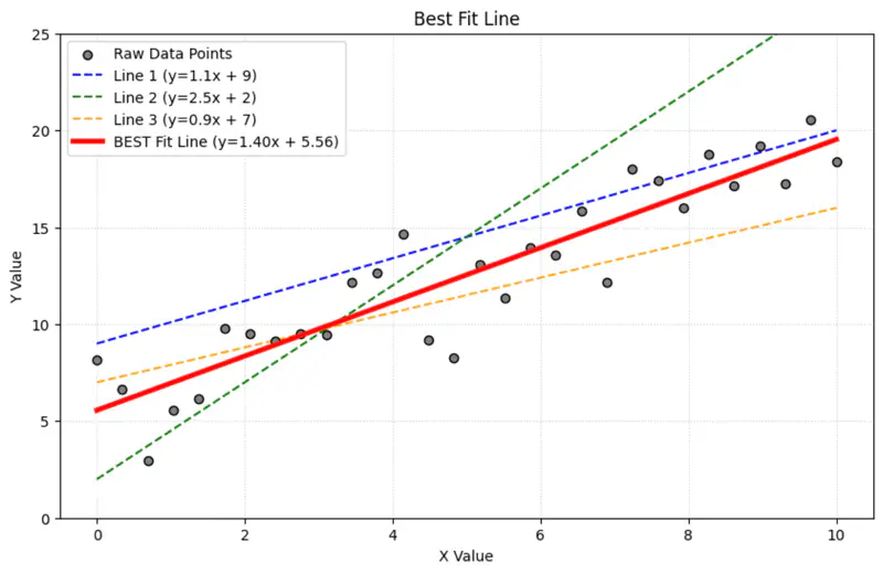
Goal 🎯 : Find the line of best fit.
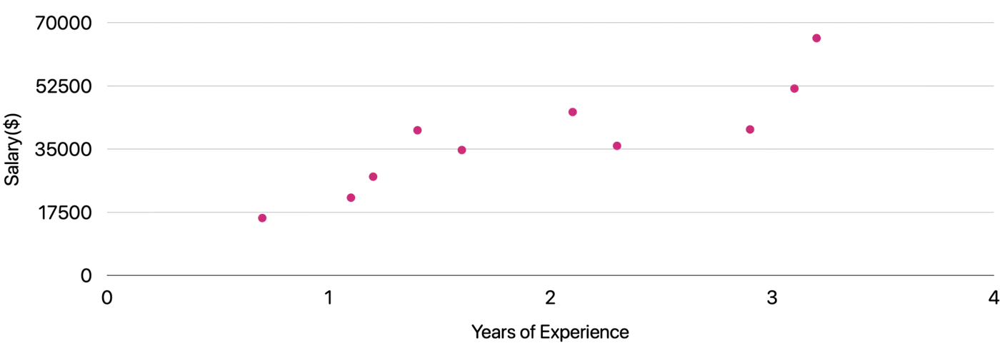
Plot: Salary vs Years of Experience
\[y = mx + c = w_1x + w_0\]Slope = \(m = w_1 \)
Intercept = \(c = w_0\)
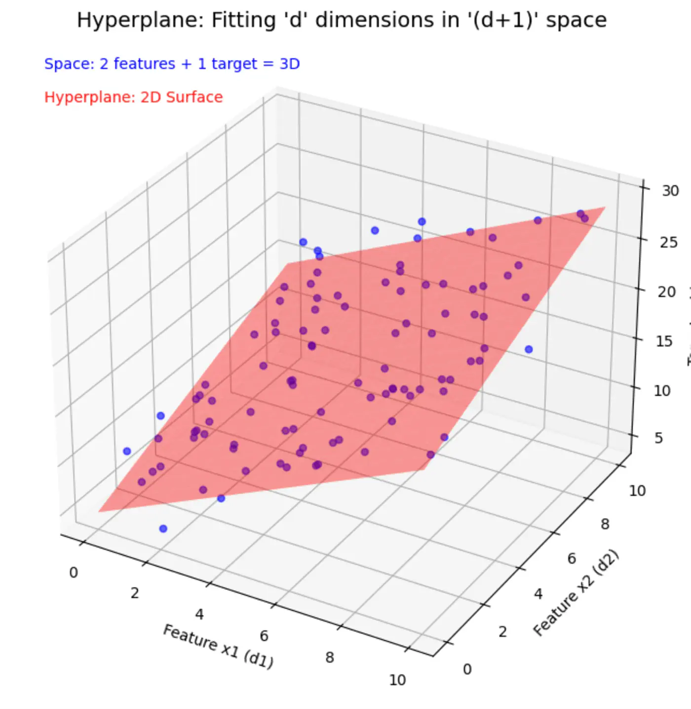
Similarly, if we include other factors/features impacting the salary 💰, such as, domain, role, etc, we get an equation of a fitting hyperplane:
\[y = w_1x_1 + w_2x_2 + \dots + w_dx_d + w_0\]where,
\[ \begin{align*} x_1 &= \text{Years of Experience} \\ x_2 &= \text{Domain (Tech, BFSI, Telecom, etc.)} \\ x_3 &= \text{Role (Dev, Tester, DevOps, ML, etc.)} \\ x_d &= d^{th} ~ feature \\ w_0 &= \text{Salary of 0 years experience} \\ \end{align*} \]Space = ’d’ features + 1 target variable = ’d+1’ dimensions
In a ’d+1’ dimensional space, we try to fit a ’d’ dimensional hyperplane.
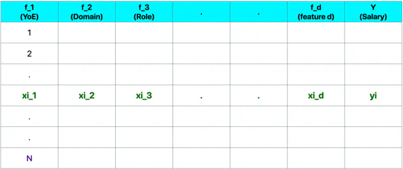
Let, data = \( {(x_i, y_i)}_{i=1}^N ; ~ x_i \in R^d , y_i \in R^d\)
where, N = number of training samples.
Note: Fitting hyperplane (\(y = w_1x_1 + w_2x_2 + \dots + w_dx_d + w_0\)) is the model.
Objective 🎯: find the parameters/weights (\(w_0, w_1, w_2, \dots w_d \)) of the model.
\(\mathbf{w} = \begin{bmatrix} w_1 \\ w_2 \\ \vdots \\ w_d \end{bmatrix}_{\text{d x 1}}\)
\( \mathbf{x_i} = \begin{bmatrix} x_{i_1} \\ x_{i_2} \\ \vdots \\ x_{i_d} \end{bmatrix}_{\text{d x 1}} \)
\( \mathbf{y} = \begin{bmatrix} y_1 \\ y_2 \\ \vdots \\ y_i \\ \vdots \\ y_n \end{bmatrix}_{\text{n x 1}} \)
\( X =
\begin{bmatrix}
x_{11} & x_{12} & \cdots & x_{1d} \\
x_{21} & x_{22} & \cdots & x_{2d} \\
\vdots & \vdots & \ddots & \vdots \\
x_{i1} & x_{i2} & \cdots & x_{id} \\
\vdots & \vdots & \ddots & \vdots \\
x_{n1} & x_{n2} & \cdots & x_{nd} \\
\end{bmatrix}
_{\text{n x d}}
\)
Prediction:
Error = Actual - Predicted
\[ \epsilon_i = y_i - \hat{y_i}\]Goal 🎯: Minimize error between actual and predicted.
We can quantify the error for a single data point in following ways:
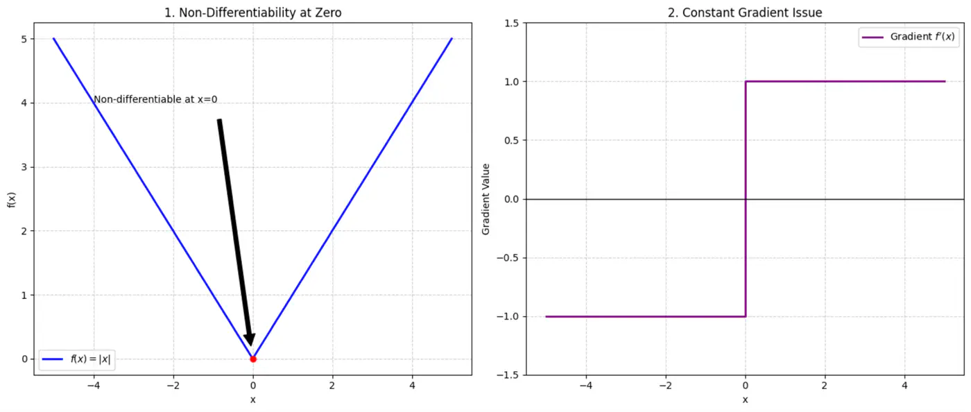
- Absolute error = \(|y_i - \hat{y_i}|\)
- Squared error = \((y_i - \hat{y_i})^2\)
Not differentiable at x=0, required for gradient descent.
Constant gradient, i.e \(\pm 1\), model learns at same rate, whether the error is large or small.
Average loss across all data points.
Mean Squared Error (MSE) =
\[ J(w) = \frac{1}{n} \sum_{i=1}^N (y_i - \hat{y_i})^2 \]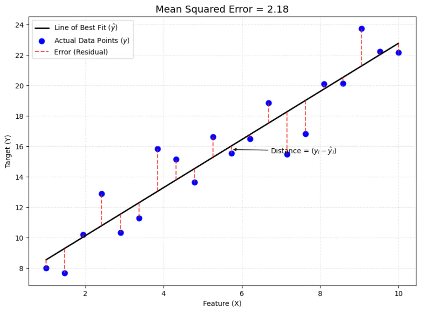
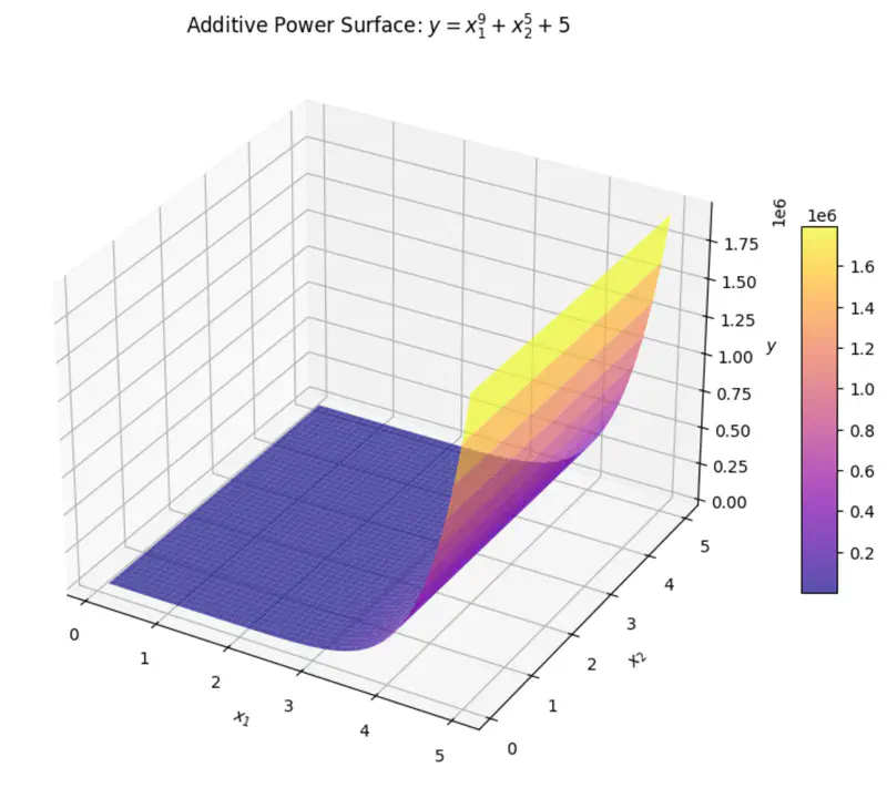
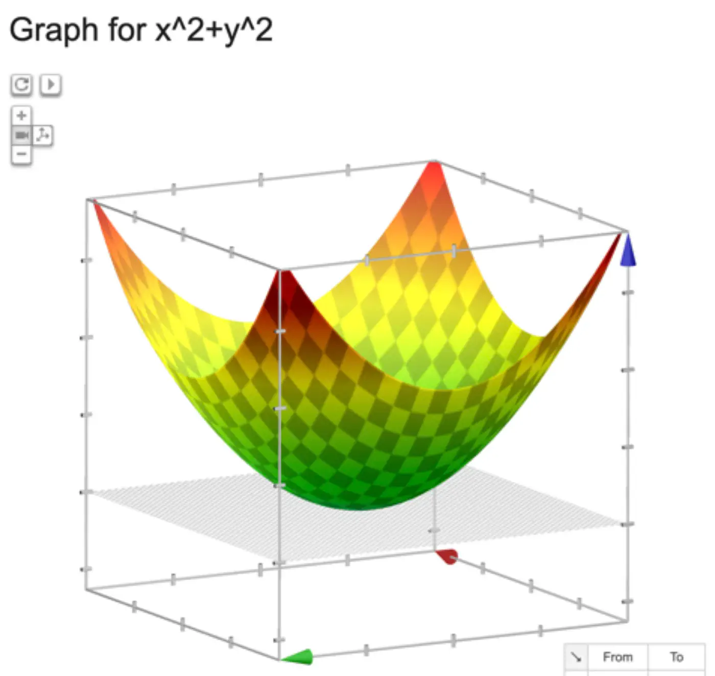
The above equation is quadratic in \(w_0, w_1, w_2, \dots w_d \).
Below is an image of a Paraboloid in 3D, similarly we will have a Paraboloid in ’d’ dimensions.
In order to find the minima of the cost function we need to take its derivative w.r.t weights and equate to 0.
\[ \begin{align*} \frac{\partial{J(w)}}{\partial{w_0}} = 0 \\ \frac{\partial{J(w)}}{\partial{w_1}} = 0 \\ \frac{\partial{J(w)}}{\partial{w_2}} = 0 \\ \vdots \\ \frac{\partial{J(w)}}{\partial{w_d}} = 0 \\ \end{align*} \]We have ‘d+1’ linear equations to solve for ‘d+1’ weights \(w_0, w_1, w_2, \dots , w_d\).
But solving ‘d+1’ system of linear equations (called the ’normal equations’) is tedious and NOT used for practical purposes.
where,
\(\mathbf{w} = \begin{bmatrix} w_1 \\ w_2 \\ \vdots \\ w_d \end{bmatrix}_{\text{d x 1}}\)
\( \mathbf{x_i} = \begin{bmatrix} x_{i_1} \\ x_{i_2} \\ \vdots \\ x_{i_d} \end{bmatrix}_{\text{d x 1}} \)
\( \mathbf{y} = \begin{bmatrix} y_1 \\ y_2 \\ \vdots \\ y_i \\ \vdots \\ y_n \end{bmatrix}_{\text{n x 1}} \)
\( X =
\begin{bmatrix}
x_{11} & x_{12} & \cdots & x_{1d} \\
x_{21} & x_{22} & \cdots & x_{2d} \\
\vdots & \vdots & \ddots & \vdots \\
x_{i1} & x_{i2} & \cdots & x_{id} \\
\vdots & \vdots & \ddots & \vdots \\
x_{n1} & x_{n2} & \cdots & x_{nd} \\
\end{bmatrix}
_{\text{n x d}}
\)
Prediction:
Let’s expand the cost function J(w):
\[ \begin{align*} J(w) &= \frac{1}{n} (y - Xw)^2 \\ &= \frac{1}{n} (y - Xw)^T(y - Xw) \\ &= \frac{1}{n} (y^T - w^TX^T)(y - Xw) \\ J(w) &= \frac{1}{n} (y^Ty - w^TX^Ty - y^TXw + w^TX^TXw) \end{align*} \]Since,\(w^TX^Ty\), is a scalar, so it is equal to its transpose.
\[ w^TX^Ty = (w^TX^Ty)^T = y^TXw\]\[ J(w) = \frac{1}{n} (y^Ty - y^TXw - y^TXw + w^TX^TXw)\]\[ J(w) = \frac{1}{n} (y^Ty - 2y^TXw + w^TX^TXw) \]Note: \(X^2 = X^TX\) and \((AB)^T = B^TA^T\)
To find the minimum, take the derivative of cost function J(w) w.r.t ‘w’, and equate to 0 vector.
\[\frac{\partial{J(w)}}{\partial{w}} = \vec{0}\]\[ \begin{align*} &\frac{\partial{[\frac{1}{n} (y^Ty - 2y^TXw + w^TX^TXw)]}}{\partial{w}} = 0\\ & \implies 0 - 2X^Ty + (X^TX + X^TX)w = 0 \\ & \implies \cancel{2}X^TXw = \cancel{2} X^Ty \\ & \therefore \mathbf{w} = (X^TX)^{-1}X^T\mathbf{y} \end{align*} \]Note: \(\frac{\partial{(a^T\mathbf{x})}}{\partial{\mathbf{x}}} = a\) and \(\frac{\partial{(\mathbf{x}^TA\mathbf{x})}}{\partial{\mathbf{x}}} = (A + A^T)\mathbf{x}\)
This is the closed-form solution of normal equations.
- Inverse may NOT exist (non-invertible).
- Time complexity of calculating the inverse is O(n^3).
If the inverse does NOT exist then we can use the approximation of the inverse, also called Pseudo Inverse or Moore Penrose Inverse (\(A^+\)).
Moore Penrose Inverse ( \(A^+\)) is calculated using Singular Value Decomposition (SVD).
SVD of \(A = U \Sigma V^T\)
Pseudo Inverse \(A^+ = V \Sigma^+ U^T\)
Where, \(\Sigma^+\) is a transpose of \(\Sigma\) with reciprocals of non-zero singular values on its diagonals.
e.g:
Note: Time Complexity = O(mn^2)
End of Section
1.4 - Probabilistic Interpretation
Error = Random Noise, Un-modeled effects
\[ \begin{align*} \epsilon_i = y_i - \hat{y_i} \\ \implies y_i = \hat{y_i} + \epsilon_i \\ \because \hat{y_i} = x_i^Tw \\ \therefore y_i = x_i^Tw + \epsilon_i \\ \end{align*} \]Actual value(\(y_i\)) = Deterministic linear predictor(\(x_i^Tw\)) + Error term(\(\epsilon_i\))
- Independent and Identically Distributed (I.I.D):
Each error term is independent of others. - Normal (Gaussian) Distributed:
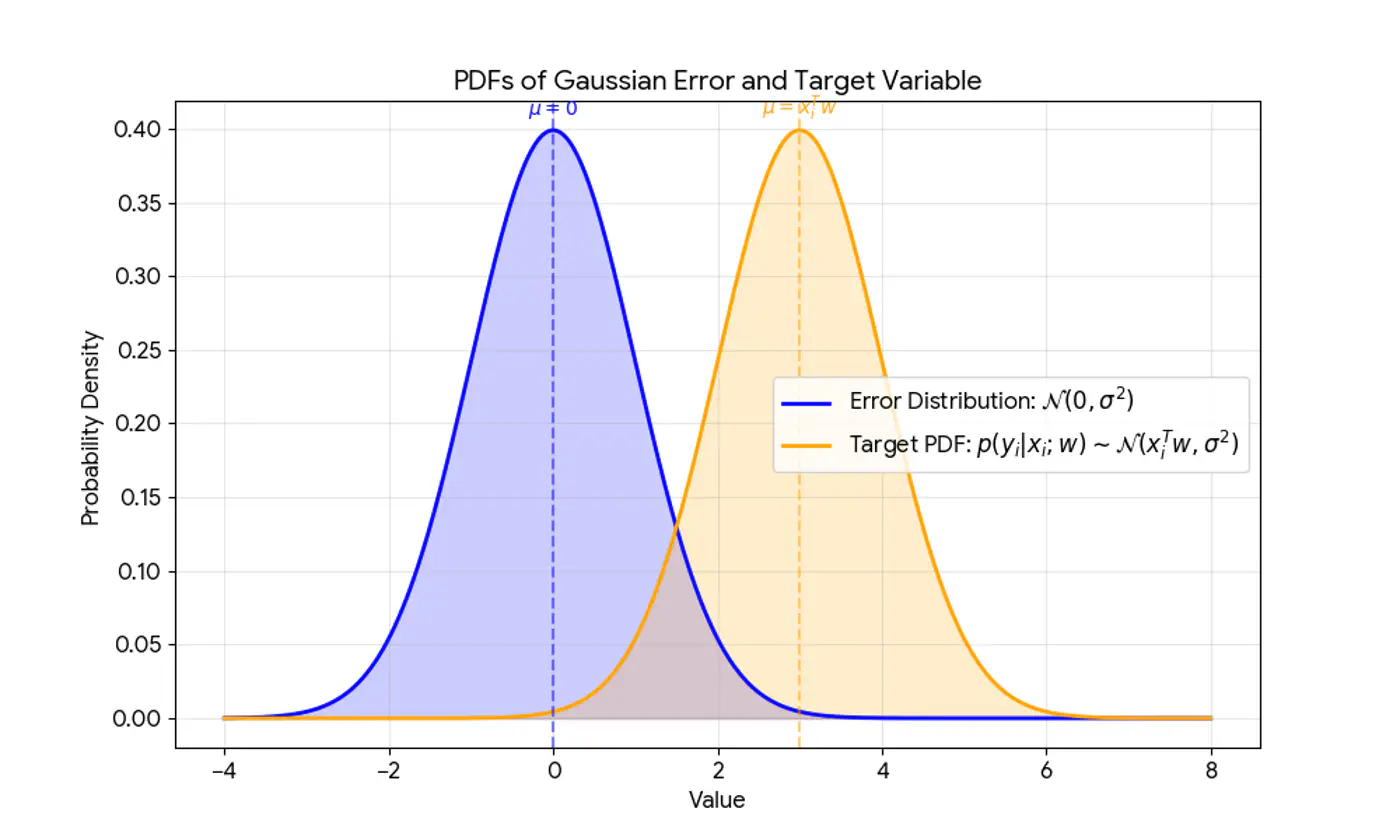
Error follows a normal distribution with mean = 0 and a constant variance, .
This implies that the target variable itself is a random variable, normally distributed around the linear relationship.
\[(y_{i}|x_{i};w)∼N(x_{i}^{T}w,\sigma^{2})\]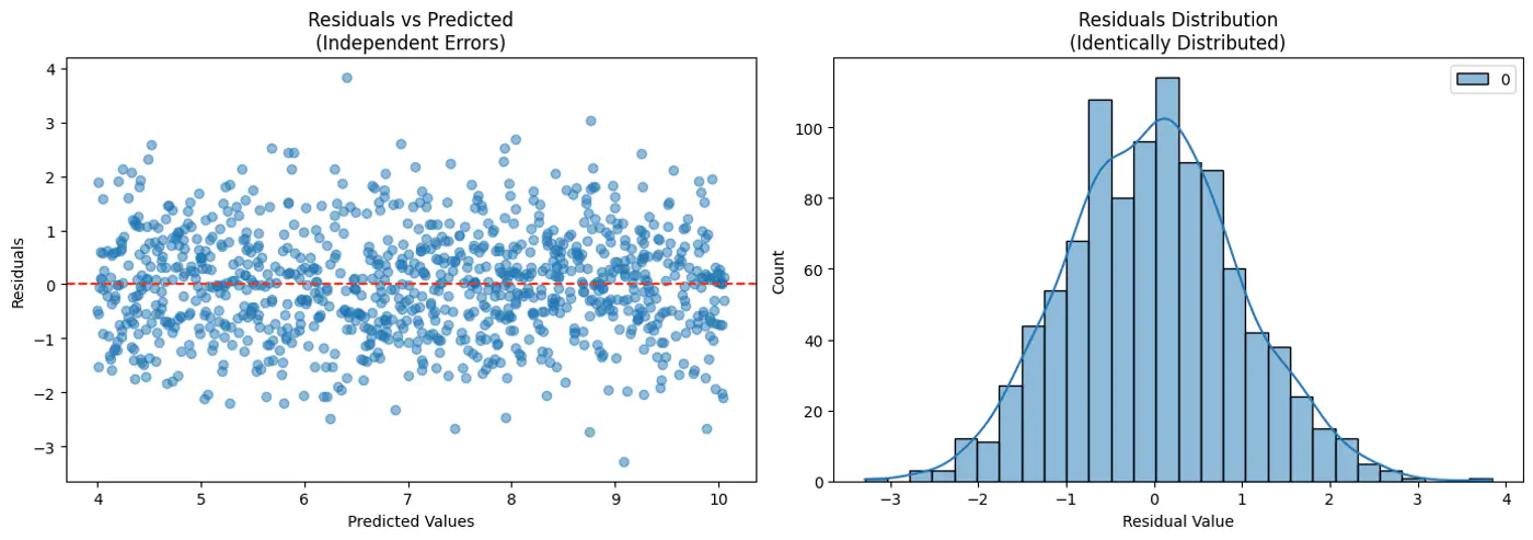
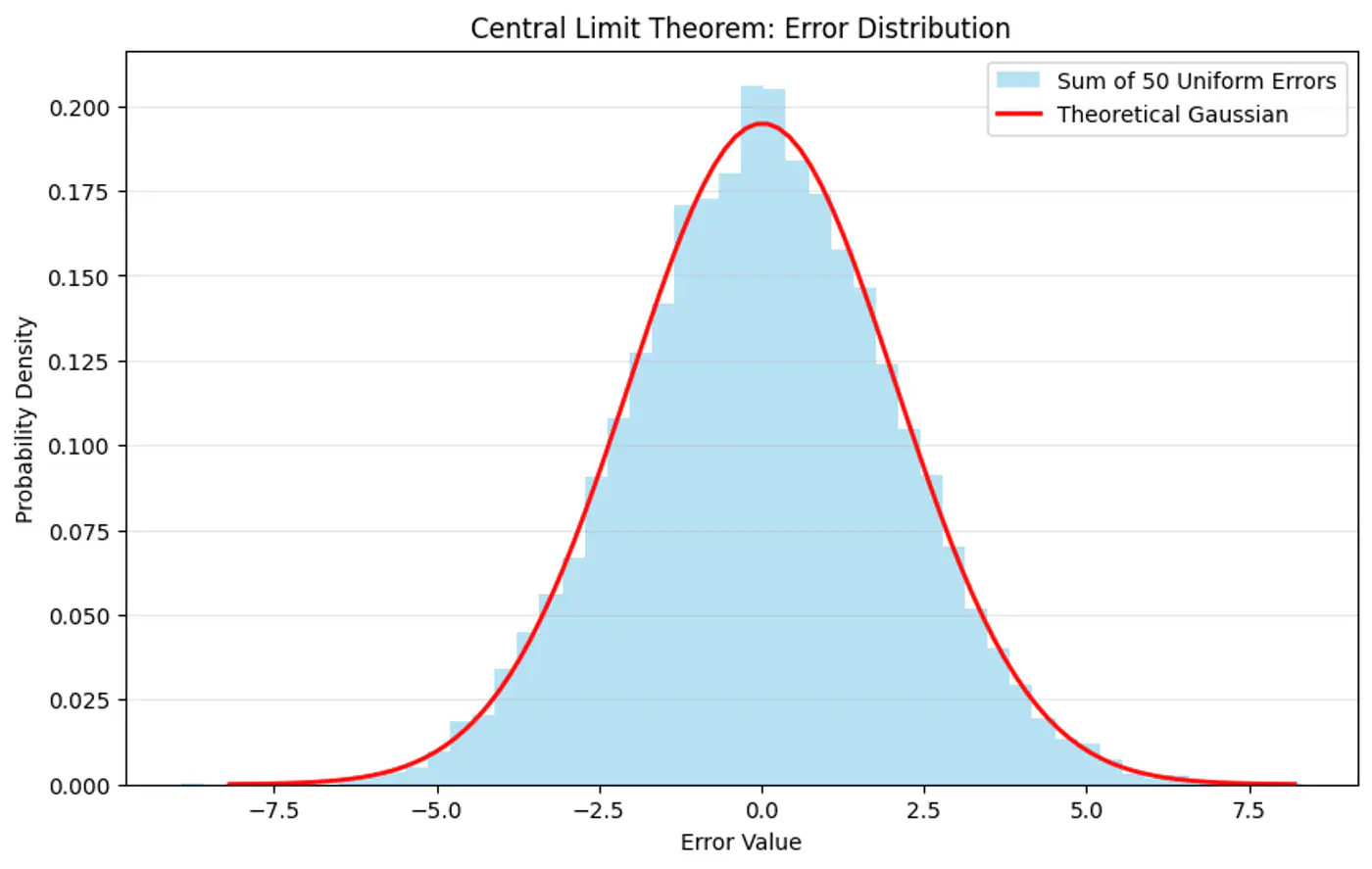
Central Limit Theorem (CLT) states that for a sequence of I.I.D random variables, the distribution of the sample mean(sum) approximates to a normal distribution, regardless of the original population distribution.
- Probability (Forward View):
Quantifies the chance of observing a specific outcome given a known, fixed model. - Likelihood (Backward/Inverse View):
Inverse concept used for inference (working backward from results to causes). It is a function of the parameters and measures how ‘likely’ a specific set of parameters makes the observed data appear.
‘Find the most plausible explanation for what I see.'
The goal of the probabilistic interpretation is to find the parameters ‘w’ that maximize the probability (likelihood) of observing the given dataset.
Assumption: Training data is I.I.D.
\[ \begin{align*} Likelihood &= \mathcal{L}(w) \\ \mathcal{L}(w) &= p(y|x;w) \\ &= \prod_{i=1}^N p(y_i| x_i; w) \\ &= \prod_{i=1}^N \frac{1}{\sigma\sqrt{2\pi}}e^{-\frac{(y_i-x_i^Tw)^2}{2\sigma^2}} \end{align*} \]Maximizing the likelihood function is mathematically complex due to the product term and the exponential function.
A common simplification is to maximize the log-likelihood function instead, which converts the product into a sum.
Note: Log is a strictly monotonically increasing function.
Note: The first term is constant w.r.t ‘w'.
So, we need to find parameters ‘w’ that maximize the log likelihood.
\[ \begin{align*} log \mathcal{L}(w) & \propto -\frac{1}{2\sigma^2} \sum_{i=1}^N (y_i-x_i^Tw)^2 \\ & \because \frac{1}{2\sigma^2} \text{ is constant} \\ log \mathcal{L}(w) & \propto -\sum_{i=1}^N (y_i-x_i^Tw)^2 \\ \end{align*} \]Maximizing the log-likelihood is equivalent to minimizing the sum of squared errors, which is the exact objective of the ordinary least squares (OLS) method.
\[ \underset{w}{\mathrm{min}}\ J(w) = \underset{w}{\mathrm{min}}\ \sum_{i=1}^N (y_i - x_i^Tw)^2 \]End of Section
1.5 - Convex Function
Refers to a property of a function where a line segment connecting any two points on its graph lies above or on the graph itself.
A convex function is curved upwards.
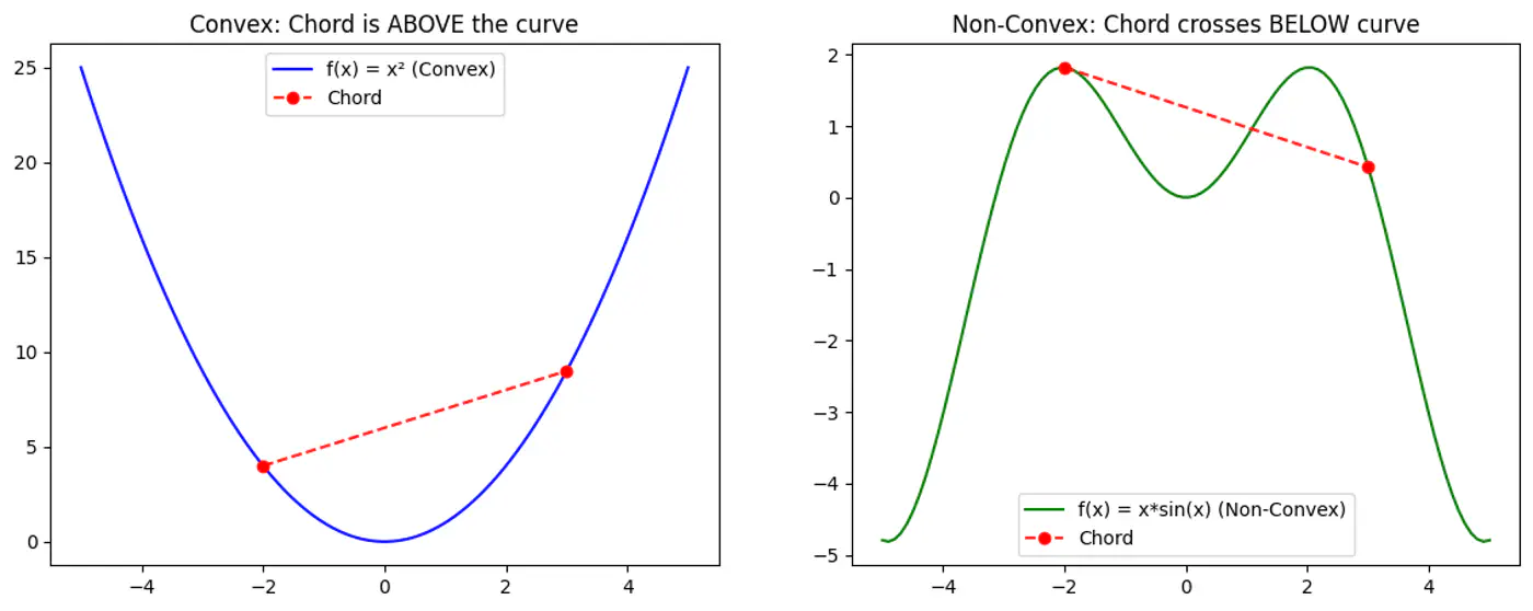
MSE cost function J(w) is convex because its Hessian (H) is always positive semi definite.
\[\nabla J(\mathbf{w})=\frac{1}{n}\mathbf{X}^{T}(\mathbf{Xw}-\mathbf{y})\]\[\mathbf{H}=\frac{\partial (\nabla J(\mathbf{w}))}{\partial \mathbf{w}^{T}}=\frac{1}{n}\mathbf{X}^{T}\mathbf{X}\]\[\therefore \mathbf{H} = \nabla^2J(w) = \frac{1}{n} \mathbf{X}^{T}\mathbf{X}\]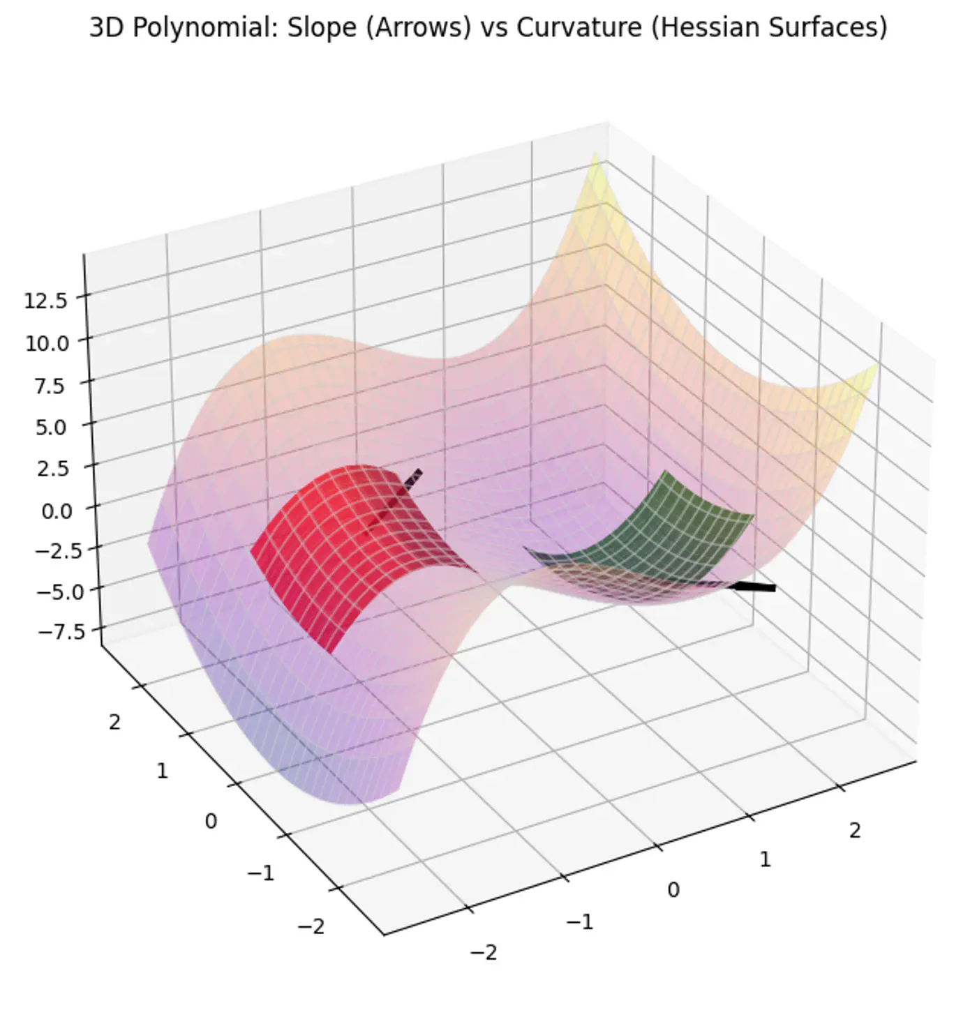
A matrix H is positive semi-definite if and only if for any non-zero vector ‘z’, the quadratic form \(z^THz \ge 0\).
For the Hessian of J(w),
\[ z^THz = z^T(\frac{1}{n}X^TX)z = \frac{1}{n}(Xz)^T(Xz) \]\((Xz)^T(Xz) = \lVert Xz \rVert^2\) = squared L2 norm (magnitude) of the vector
Note: The squared norm of any real-valued vector is always \(\ge 0\).
End of Section
1.6 - Gradient Descent
Minimize the cost 💰function.
\[J(w)=\frac{1}{2n}(y-Xw)^{2}\]Note: The 1/2 term is included simply to make the derivative cleaner (it cancels out the 2 from the square).
Normal Equation (Closed-form solution) jumps straight to the optimal point in one step.
\[w=(X^{T}X)^{-1}X^{T}y\]But it is not always feasible and computationally expensive 💰(due to inverse calculation 🧮)
An iterative optimization algorithm slowly nudges parameters ‘w’ towards a value that minimize the cost💰 function.
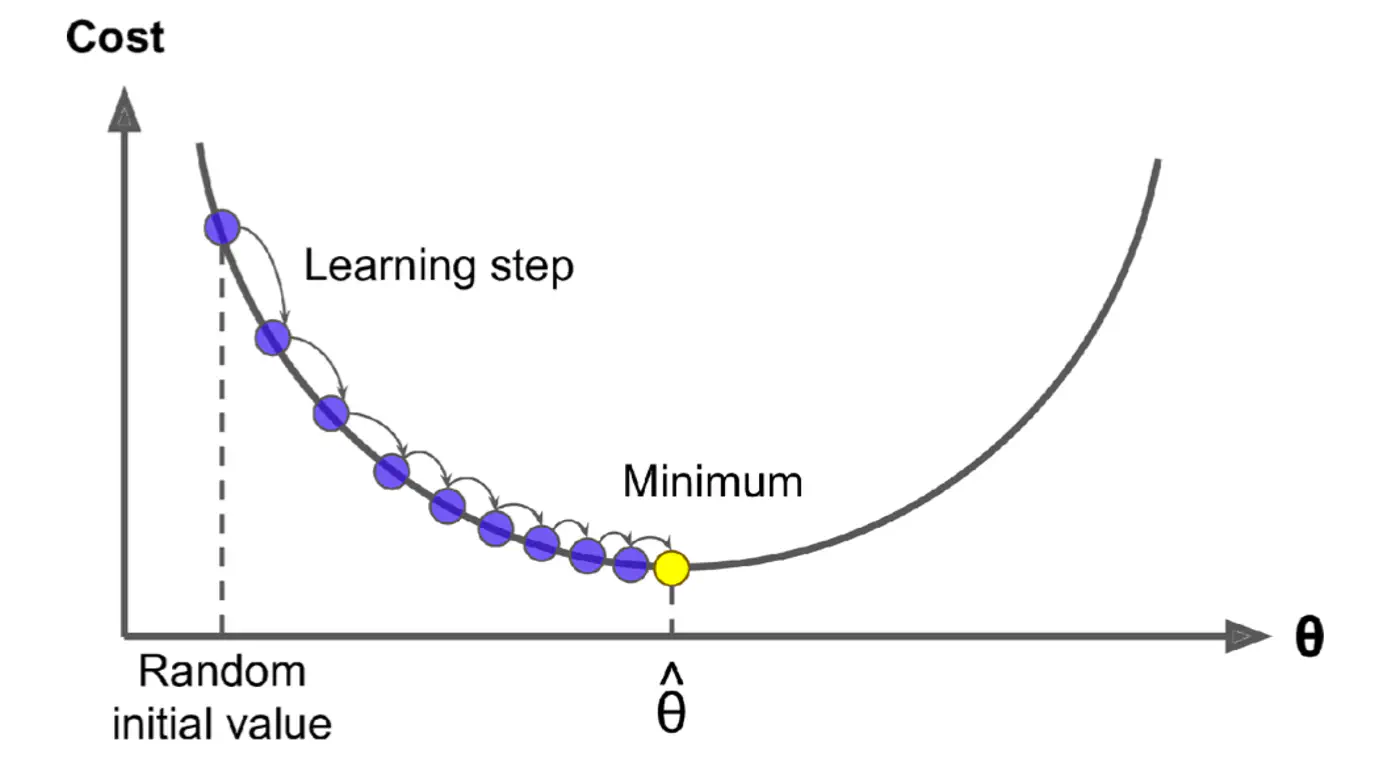
- Initialize the weights/parameters with random values.
- Calculate the gradient of the cost function at current parameter values.
- Update the parameters using the gradient. \[ w_{new} = w_{old} - \eta \frac{\partial{J(w)}}{\partial{w_{old}}} \] \( \eta \) = learning rate or step size to take for each parameter update.
- Repeat 🔁 steps 2 and 3 iteratively until convergence (to minima).
Applying chain rule:
\[ \begin{align*} &\text{Let } u = (y - Xw) \\ &\text{Derivative of } u^2 \text{ w.r.t 'w' }= 2u.\frac{\partial{u}}{\partial{w}} \\ \frac{\partial{(\frac{1}{2n} (y - Xw)^2)}}{\partial{w}} &= \frac{1}{\cancel2n}.\cancel2(y - Xw).\frac{\partial{(y - Xw)}}{\partial{w}} \\ &= \frac{1}{n}(y - Xw).X^T.(-1) \\ \therefore \frac{\partial{J(w)}}{\partial{w}} &= \frac{1}{n}X^T(Xw - y) \end{align*} \]Note: \(\frac{∂(a^{T}x)}{∂x}=a\)
Update parameter using gradient:
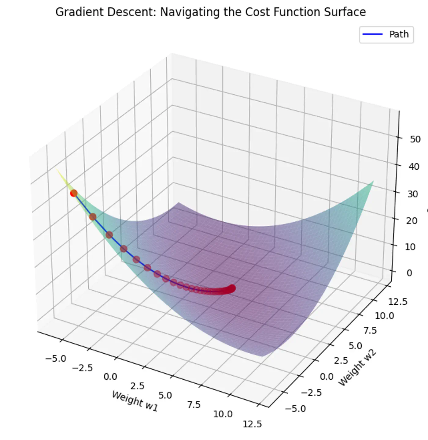
\[ w_{new} = w_{old} - \eta'. X^T(Xw - y) \]- Most important hyper parameter of gradient descent.
- Dictates the size of the steps taken down the cost function surface.
Small \(\eta\) ->
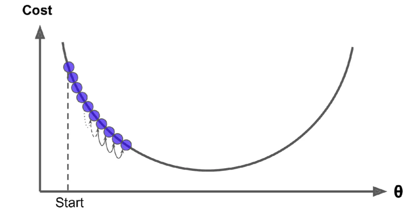
Large \(\eta\) ->
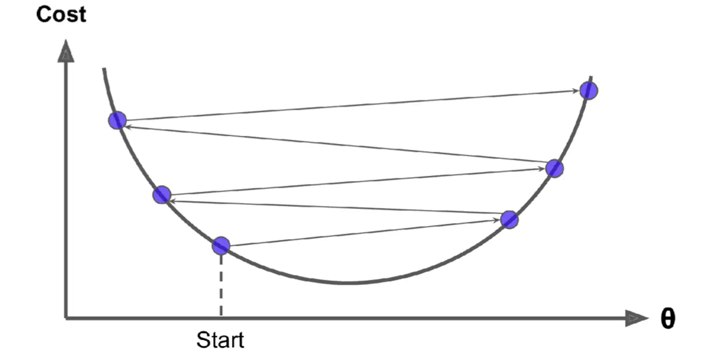
- Learning Rate Schedule:
The learning rate is decayed (reduced) over time.
Large steps initially and fine-tuning near the minimum, e.g., step decay or exponential decay. - Adaptive Learning Rate Methods:
Automatically adjust the learning rate for each parameter ‘w’ based on the history of gradients.
Preferred in modern deep learning as they require less manual tuning, e.g., Adagrad, RMSprop, and Adam.
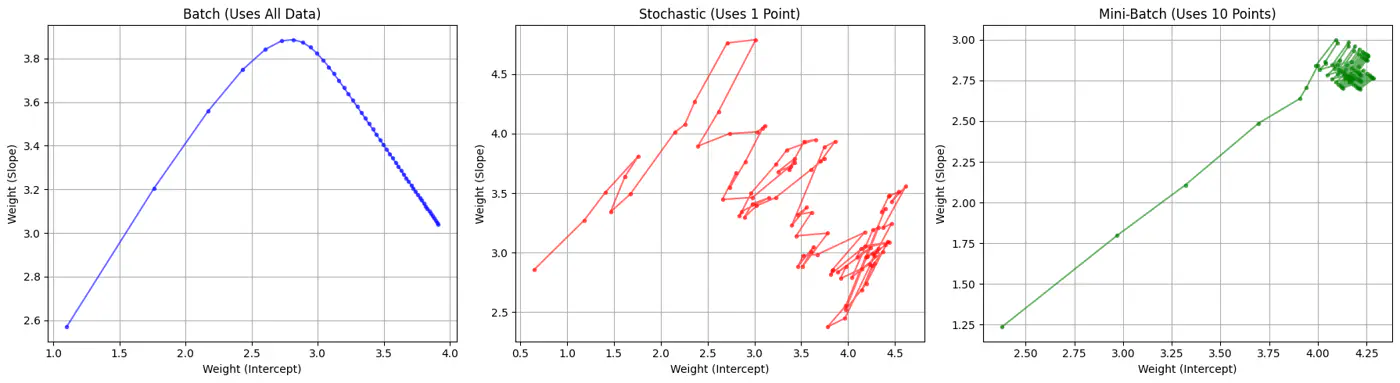
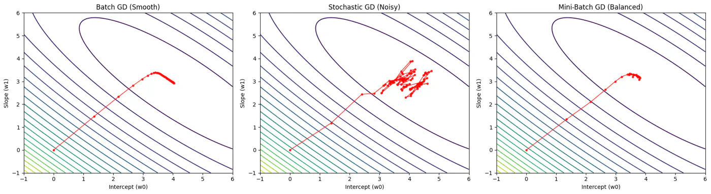
Batch, Stochastic, Mini-Batch are classified by data usage for gradient calculation in each iteration.
- Batch Gradient Descent (BGD): Entire Dataset
- Stochastic Gradient Descent (SGD): Random Point
- Mini-Batch Gradient Descent (MBGD): Subset
Computes the gradient using all the data points in the dataset for parameter update in each iteration.
\[w_{new} = w_{old} - \eta.\text{(average of all ’n’ gradients)}\]🔑Key Points:
- Slow 🐢 steps towards convergence, i.e, TC = O(n).
- Smooth, direct path towards minima.
- Minimum number of steps/iterations.
- Not suitable for large datasets; impractical for Deep Learning, as n = millions/billions.
Uses only 1 data point selected randomly from dataset to compute gradient for parameter update in each iteration.
\[w_{new} = w_{old} - \eta.\text{(gradient at any random data point)}\]🔑Key Points:
- Computationally fastest 🐇 per step; TC = O(1).
- Highly noisy, zig-zag path to minima.
- High variance in gradient estimation makes path to minima volatile, requiring a careful decay of learning rate to ensure convergence to minima.
- Uses small randomly selected subsets of dataset, called mini-batch, (1<k<n), to compute gradient for parameter update in each iteration. \[w_{new} = w_{old} - \eta.\text{(average gradient of ‘k' data points)}\]
🔑Key Points:
- Moderate time ⏰ consumption per step; TC = O(k<n).
- Less noisy, and more reliable convergence than stochastic gradient descent.
- More efficient and faster than batch gradient descent.
- Standard optimization algorithm for Deep Learning.Note: Vectorization on GPUs allows for parallel processing of mini-batches; also GPUs are the reason for the mini-batch size to be a power of 2.
End of Section
1.7 - Polynomial Regression
We can use a linear model to fit non-linear data.
Add powers of each feature as new features, then train a linear model on this extended set of features.
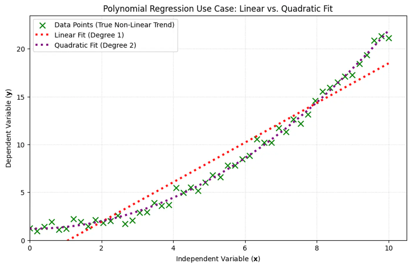
Linear: \(\hat{y_i} = w_0 + w_1x_{i_1} \)
Polynomial (quadratic): \(\hat{y_i} = w_0 + w_1x_{i_1} + w_2x_{i_1}^2\)
Polynomial (n-degree): \(\hat{y_i} = w_0 + w_1x_{i_1} + w_2x_{i_1}^2 +w_3x_{i_1}^3 + \dots + w_nx_{i_1}^n \)
Above polynomial can be re-written as linear equation:
\[\hat{y_i} = w_0 + w_1X_1 + w_2X_2 +w_3X_3 + \dots + w_nX_n \]where, \(X_1 = x_{i_1}, X_2 = x_{i_1}^2, X_3 = x_{i_1}^3, \dots, X_n = x_{i_1}^n\)
=> the model is still linear w.r.t to its parameters/weights \(w_0, w_1, w_2, \dots , w_n \).
e.g:
- Fit a linear model to the data points.
- Plot the errors.
- If the variance of errors is too high, then try polynomial features.
Note: Detect and remove outliers from error distribution.

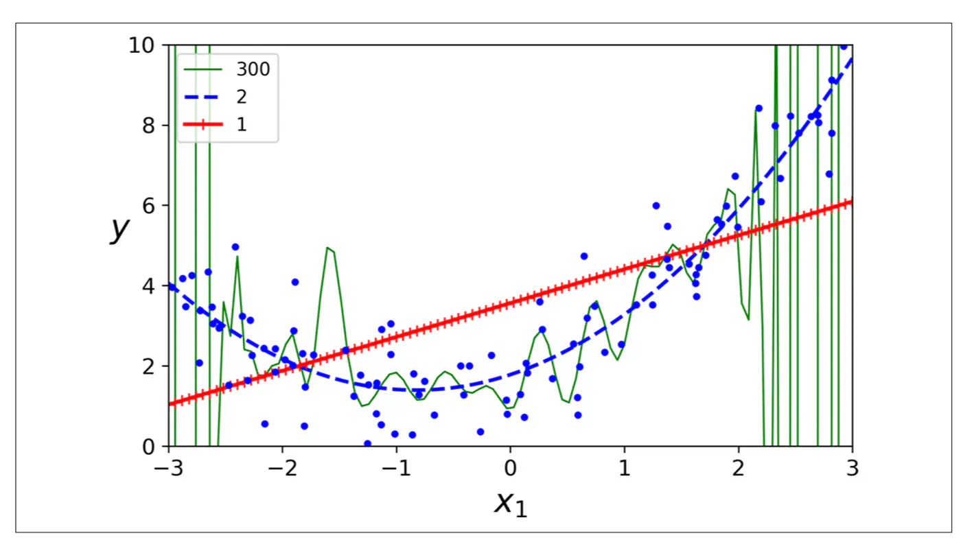
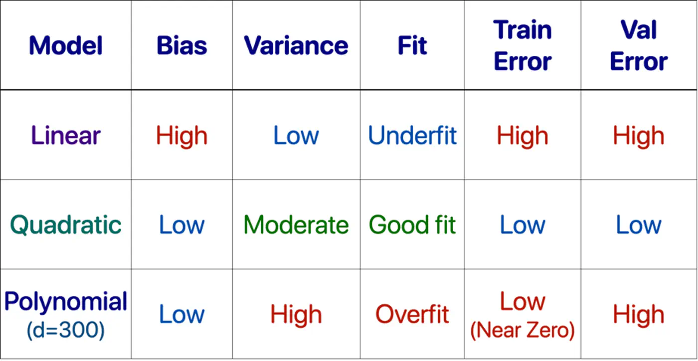
- Polynomial model : Over-fitting ❌
- Linear model : Under-fitting ❌
- Quadratic model: Generalizes best ✅
End of Section
1.8 - Data Splitting
- Training Data: Learn model parameters (Textbook + Practice problems)
- Validation Data: Tune hyper-parameters (Mock tests)
- Test Data: Evaluate model performance (Real (final) exam)
Data leakage occurs when information from the validation or test set is inadvertently used to train 🏃♂️ the model.
The model ‘cheats’ by learning to exploit information it should not have access to, resulting in artificially inflated performance metrics during testing 🧪.
- Small datasets(1K-100K): 60/20/20, 70/15/15 or 80/10/10
- Large datasets(>1M): 98/1/1 would suffice, as 1% of 1M is still 10K.
Note: There is no fixed rule, its trial and error.
If there is class imbalance in the dataset, (e.g., 95% class A , 5% class B), a random split might result in the validation set having 99% class A.
Solution: Use stratified sampling to ensure class proportions are maintained across all splits (train️/validation/test).
Note: Non-negotiable for imbalanced data.
- In time-series ⏰ data, divide the data chronologically, not randomly, i.e, training data time ⏰ should precede validation data time ⏰.
- We always train 🏃♂️ on past data to predict future data.
Golden rule: Never look 👀 into the future.
End of Section
1.9 - Cross Validation
Do not trust one split of the data; validate across many splits, and average the result to reduce randomness and bias.
Note: Two different splits of the same dataset can give very different validation scores.
Cross-validation is a statistical resampling technique used to evaluate how well a machine learning model generalizes to an independent, unseen dataset.
It works by systematically partitioning the available data into multiple subsets, or ‘folds’, and then training and testing the model on different combinations of these folds.
- K-Fold Cross-Validation
- Leave-One-Out Cross-Validation (LOOCV)
- Shuffle the dataset randomly (except time-series ⏳).
- Split data into k equal subsets(folds).
- Iterate through each unique fold, using it as the validation set.
- Use remaining k-1 fold for training 🏃♂️.
- Take an average of the results.Note: Common choice for k=5 or 10.
- Iteration 1: [V][T][T][T][T]
- Iteration 2: [T][V][T][T][T]
- Iteration 3: [T][T][V][T][T]
- Iteration 4: [T][T][T][V][T]
- Iteration 5: [T][T][T][T][V]
Model is trained 🏃♂️on all data points except one, and then tested 🧪on that remaining single observation.
LOOCV is an extreme case of k-fold cross-validation, where, k=n (number of data points).
Pros:
Useful for small (<1000) datasets.Cons:
Computationally 💻 expensive 💰.
End of Section
1.10 - Bias Variance Tradeoff
Mean Squared Error (MSE) = \(\frac{1}{n} \sum_{i=1}^n (y_i - \hat{y_i})^2\)
Total Error = Bias^2 + Variance + Irreducible Error
- Bias = Systematic Error
- Bias measures how far the average prediction of a model is from the true value.
- Variance = Sensitivity to Data
- Variance measures how much the predictions of a model vary for different training datasets.
- Irreducible Error = Sensor noise, Human randomness
- Inherent uncertainty in the data generation process itself and cannot be reduced by any model.
Systematic error from overly simplistic assumptions or strong opinion in the model.
e.g. House 🏠 prices 💰 = Rs. 10,000 * Area (sq. ft).
Note: This is over simplified view, because it ignores, amenities, location, age, etc.
Error from sensitivity to small fluctuations 📈 in the data.
e.g. Deep neural 🧠 network trained on a small dataset.
Note: Memorizes everything, including noise.
Say a house 🏠 in XYZ street was sold for very low price 💰.
Reason: Distress selling (outlier), or incorrect entry (noise).
Note: Model will make wrong(lower) price 💰predictions for all houses in XYZ street.
Goal 🎯 is to minimize total error.
Find a sweet-spot balance ⚖️ between Bias and Variance.
A good model ‘generalizes’ well, i.e.,
- Is not too simple or has a strong opinion.
- Does not memorize 🧠 everything in the data, including noise.
- Make model more complex.
- Add more features, add polynomial features.
- Decrease Regularization.
- Train 🏃♂️longer, the model has not yet converged.
- Add more data (most effective).
- Harder to memorize 🧠 1 million examples than 100.
- Use data augmentation, if getting more data is difficult.
- Increase Regularization.
- Early stopping 🛑, prevents memorization 🧠.
- Dropout (DL), randomly kill neurons, prevents co-adaptation.
- Use Ensembles.
- Averaging reduces variance.
Note: Co-adaptation refers to a phenomenon where neurons in a neural network become highly dependent on each other to detect features, rather than learning independently.
End of Section
1.11 - Regularization
Over-Fitting happens when we have a complex model that creates highly erratic curve to fit every single data point, including the random noise.
- Excellent performance on training 🏃♂️ data, but poor performance on unseen data.
- Penalty for overly complex models, i.e, models with excessively large or numerous parameters.
- Focus on learning general patterns rather than memorizing 🧠 everything, including noise in training 🏃♂️data.
Set of techniques that prevents over-fitting by adding a penalty term to the model’s loss function.
\[ J_{reg}(w) = J(w) + \lambda.\text{Penalty(w)} \]\(\lambda\) = Regularization strength hyper parameter, bias-variance tradeoff knob.
- High \(\lambda\): High ⬆️ penalty, forces weights towards 0, simpler model.
- Low \(\lambda\): Weak ⬇️ penalty, closer to un-regularized model.
- By intentionally simplifying a model (shrinking weights) to reduce its complexity, which prevents it from overfitting.
- Penalty pulls feature weights closer to zero, making the model less faithful representation of the training data’s true complexity.
- L2 Regularization (Ridge Regression)
- L1 Regularization (Lasso Regression)
- Elastic Net Regularization
- Early Stopping
- Dropout (Neural Networks)
- Penalty term: \(\ell_2\) norm - penalizes large weights quadratically.
- Pushes the weights close to 0 (not exactly 0), making models more stable by distributing importance across weights.
- Splits feature importance across co-related features.
- Use case: Best when most features are relevant and co-related.
- Also known as Ridge regression or Tikhonov regularization.
- Penalty term: \(\ell_1\) norm.
- Shrinks some weights exactly to 0, effectively performing feature selection, giving sparse solutions.
- For a group of highly co-related features, arbitrarily selects one feature and shrinks others to 0.
- Use case: Best when using high-dimensional datasets (d»n) where we suspect many features are irrelevant or redundant, or when model interpretability matters.
- Also known as Lasso (Least Absolute Shrinkage and Selection Operator) regression.
- Computational hack: \(\frac{\partial{|w_j|}}{\partial{w_j}} = 0\), since absolute function is not differentiable at 0.
- Penalty term : linear combination of and norm.
- Sparsity(feature-selection) of L1 and stability/grouping effect of L2 regularization.
- Use case: Best when we have high dimensional data with correlated features and we want sparse and stable solution.
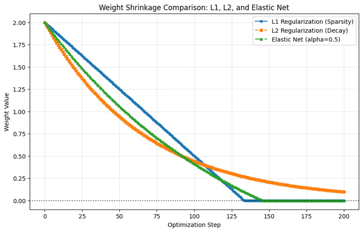
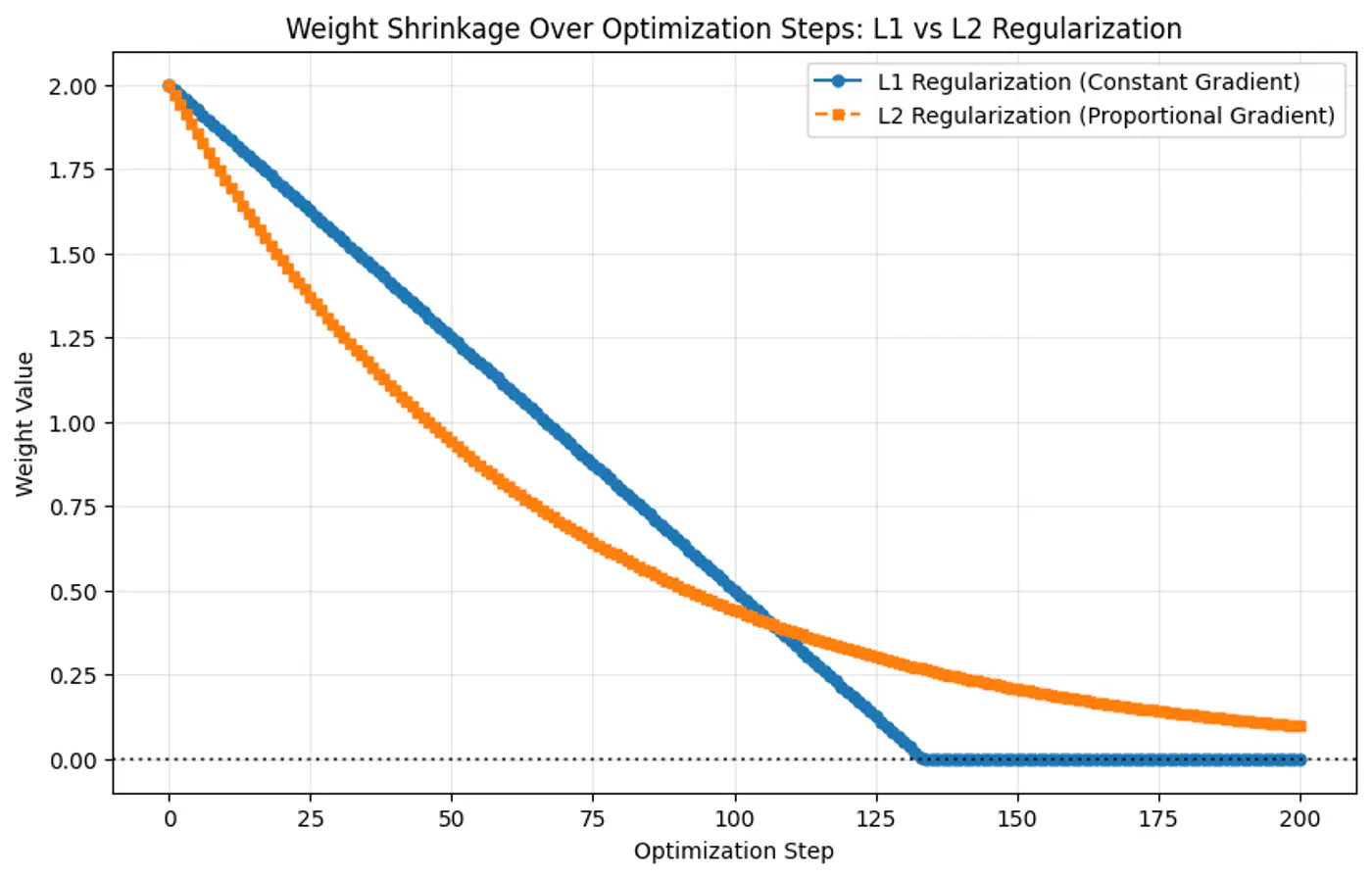
- Because the gradient of L1 penalty (absolute function) is a constant value, i.e, \(\pm 1\), this means a constant reduction in weight at each step, making it gradually reach to 0 in finite steps.
- Whereas, the derivative of L2 penalty is proportional to the weight (\(2w_j\)) and as the weight reaches close to 0, the gradient also becomes very small, this means that the weight will become very close to 0, but not exactly equal to 0.
End of Section
1.12 - Regression Metrics
MAE = \(\frac{1}{n} \sum_{i=1}^n |y_i - \hat{y_i}|\)
- Treats each error equally.
- Robust to outliers.
- Not differentiable x=0.
- Using gradient descent requires computational hack.
- Easy to interpret, as same units as target variable.
MSE = \(\frac{1}{n} \sum_{i=1}^n (y_i - \hat{y_i})^2\)
- Heavily penalizes large errors.
- Sensitive to outliers.
- Differentiable everywhere.
- Used by gradient descent and most other optimization algorithms.
- Difficult to interpret, as it has squared units.
RMSE = \(\sqrt{\frac{1}{n} \sum_{i=1}^n (y_i - \hat{y_i})^2}\)
- Easy to interpret, as it has same units as target variable.
- Useful when we need outlier-sensitivity of MSE but the interpretability of MAE.
Measures improvement over mean model.
\[ R^2 = 1 - \frac{SS_{res}}{SS_{tot}} = 1 - \frac{\sum_{i=1}^n (y_i - \hat{y_i})^2}{\sum_{i=1}^n (y_i - \bar{y_i})^2} \]Good R^2 value depends upon the use case, e.g. :
- Car 🚗 sale, R =0.8 is good enough.
- Cancer 🧪 prediction R 0.95, as life depends on it.
Range of values:
- Best value = 1
- Baseline value = 0
- Worst value = \(- \infty\)
Note: Example for bad model is all the points lie along x-axis and model predicts y-axis.
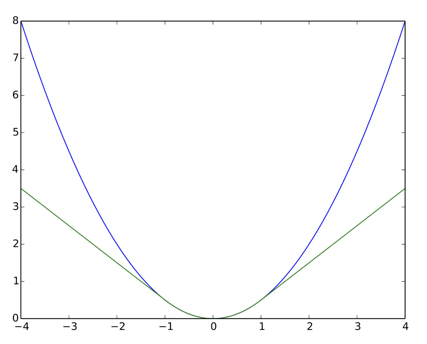
Quadratic for small errors; Linear for large errors.
\[ L_{\delta}(y, \hat{y}) = \begin{cases} \frac{1}{2}(y - \hat{y})^2 & \text{for } |y - \hat{y}| \le \delta \\ \\ \delta (|y - \hat{y}| - \frac{1}{2}\delta) & \text{otherwise} \end{cases} \]- Robust to outliers.
- Differentiable at 0; smooth convergence to minima.
- Delta (\(\delta\)) knob(hyper parameter) to control.
- \(\delta\) high: MSE
- \(\delta\) low: MAE
Note: Tune \(\delta\): MAE, for outliers > \(\delta\); MSE, for small errors < \(\delta\).
e.g: = 95th percentile of errors or 1.35\(\sigma\) for standard Gaussian data.
Huber loss (Green) and Squared loss (blue)
End of Section
1.13 - Assumptions
Linear Regression works reliably only when certain key 🔑 assumptions about the data are met.
- Linearity
- Independence of Errors (No Auto-Correlation)
- Homoscedasticity (Equal Variance)
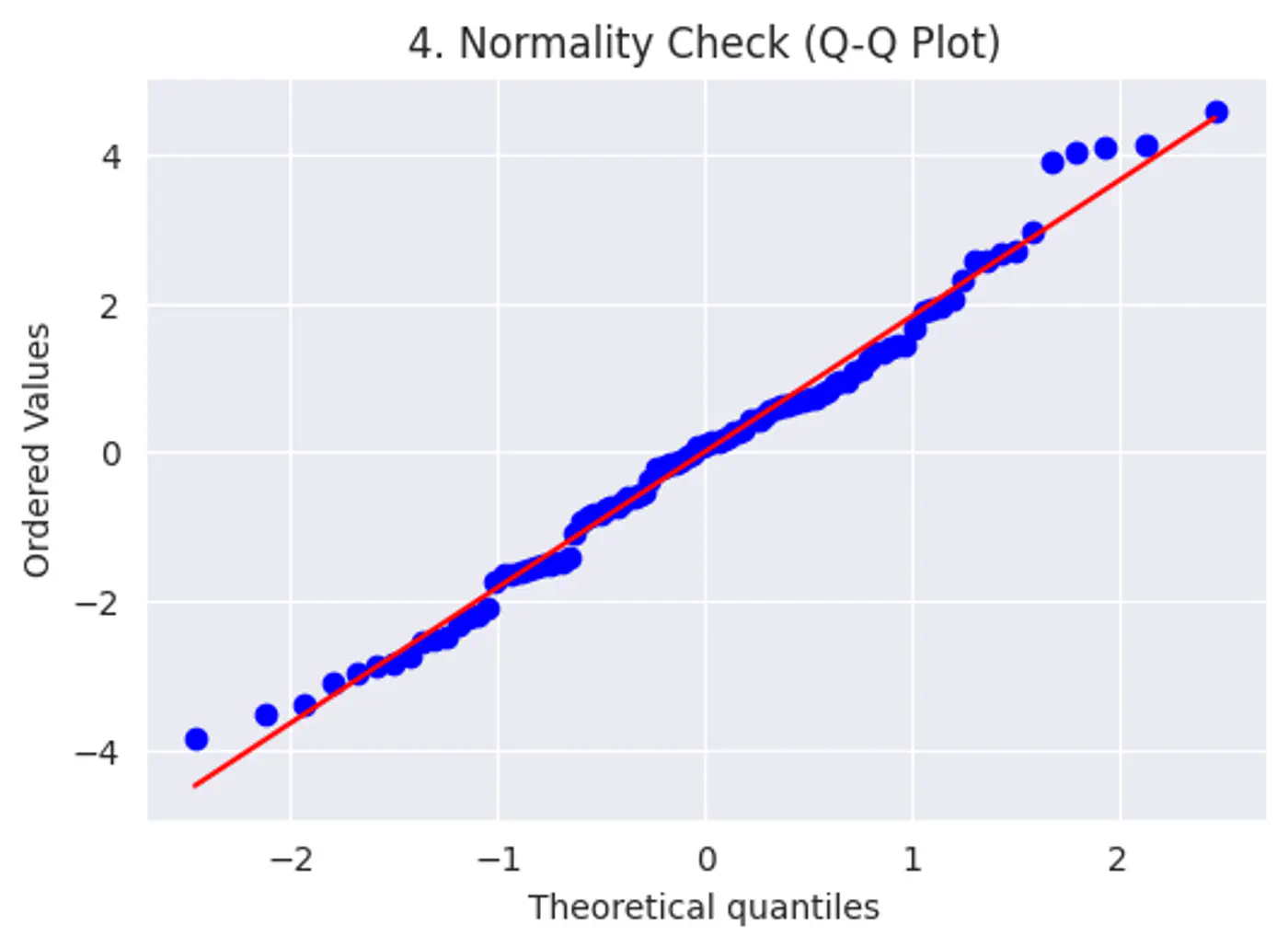
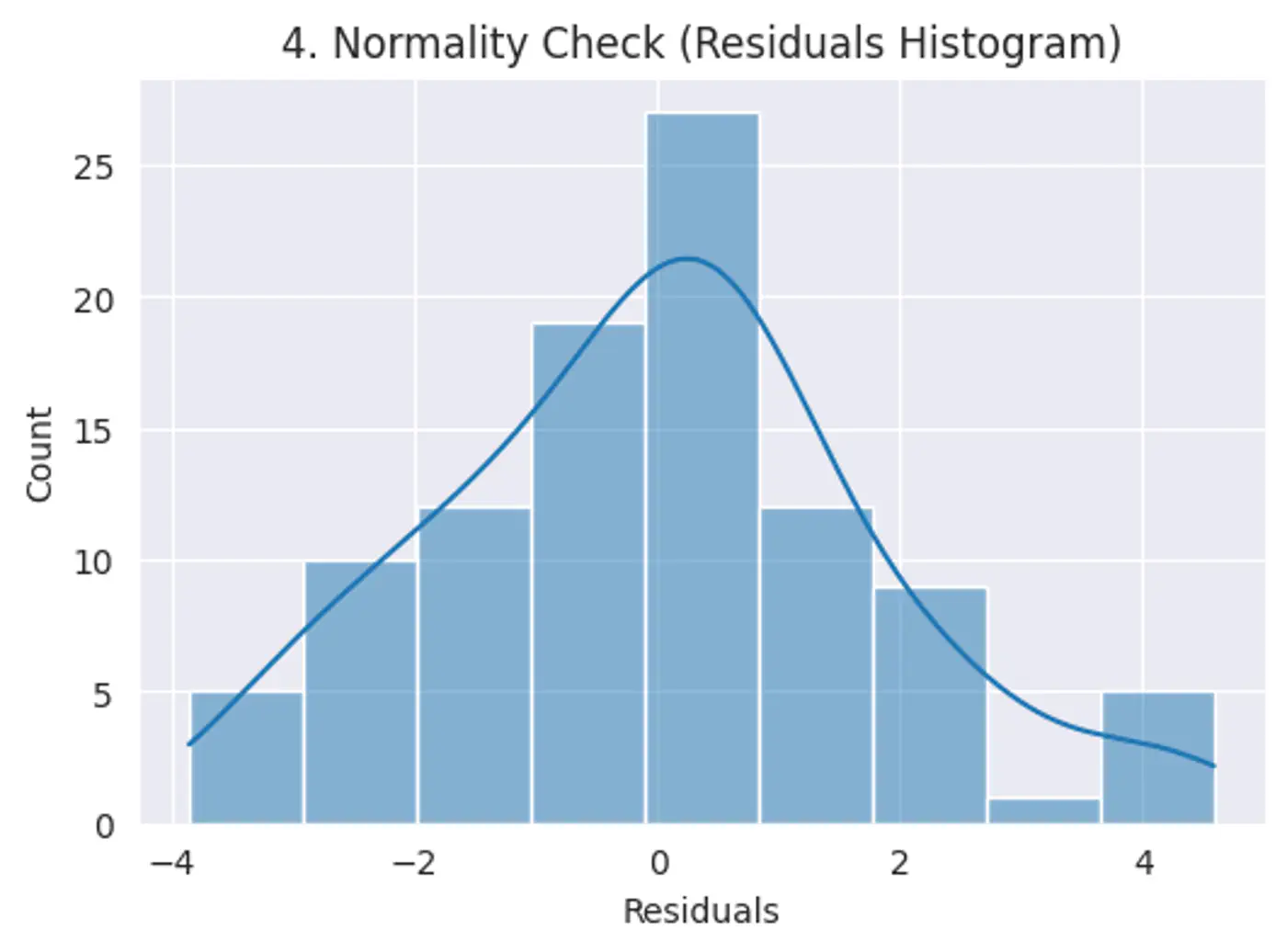
- Normality of Errors
- No Multicollinearity
- No Endogeneity (Target not correlated with the error term)
Relationship between features and target 🎯 is linear in parameters.
Note: Polynomial regression is linear regression.
\(y=w_0 +w_1x_1+w_2x_2^2 + w_3x_3^3\)
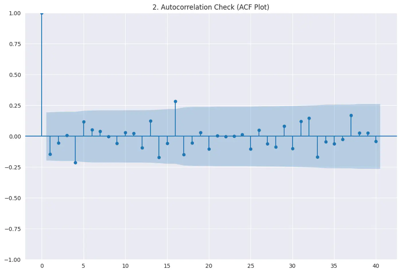
Residuals (errors) should not have a visible pattern or correlation with one another (most common in time-series ⏰ data).
Risk:
If errors are correlated, standard errors will be underestimated, making variables look ‘statistically significant’ when they are not.
Test:
Durbin–Watson test
Autocorrelation plots (ACF)
Residuals vs time
Constant variance of errors; Var(ϵ|X)=σ
Risk:
Standard errors become biased, leading to unreliable hypothesis tests (t-tests, F-tests).
Test:
- Breusch–Pagan test
- White test
Fix:
- Log transform
- Weighted Least Squares(WLS)
Error terms should follow a normal distribution; (Required for small datasets.)
Note: Because of Central Limit Theorem, with a large enough sample size, this becomes less critical for estimation.
Risk: Hypothesis testing (calculating p-values and confidence intervals), we assume the error terms follow a normal distribution.
Test:
Q-Q plot
Shapiro-Wilk Test
Features should not be highly correlated with each other.
Risk:
- High correlation makes it difficult to determine the unique, individual impact of each feature. This leads to high variance in model parameter estimates, small changes in data cause large swings in parameters.
- Model interpretability issues.
Test:
- Variance Inflation Factor(VIF)VIF > 5 → concern, VIF > 10 → serious issue
Fix:
- PCA
- Remove redundant features
Error term must be uncorrelated with the features; E[ϵ|X] = 0
Risk:
- Parameters will be biased and inconsistent.
Test:
- Hausman Test
- Durbin-Wu-Hausman (DWH) Test
Fix:
- Controlled experiments.
End of Section
2.1 - Binary Classification
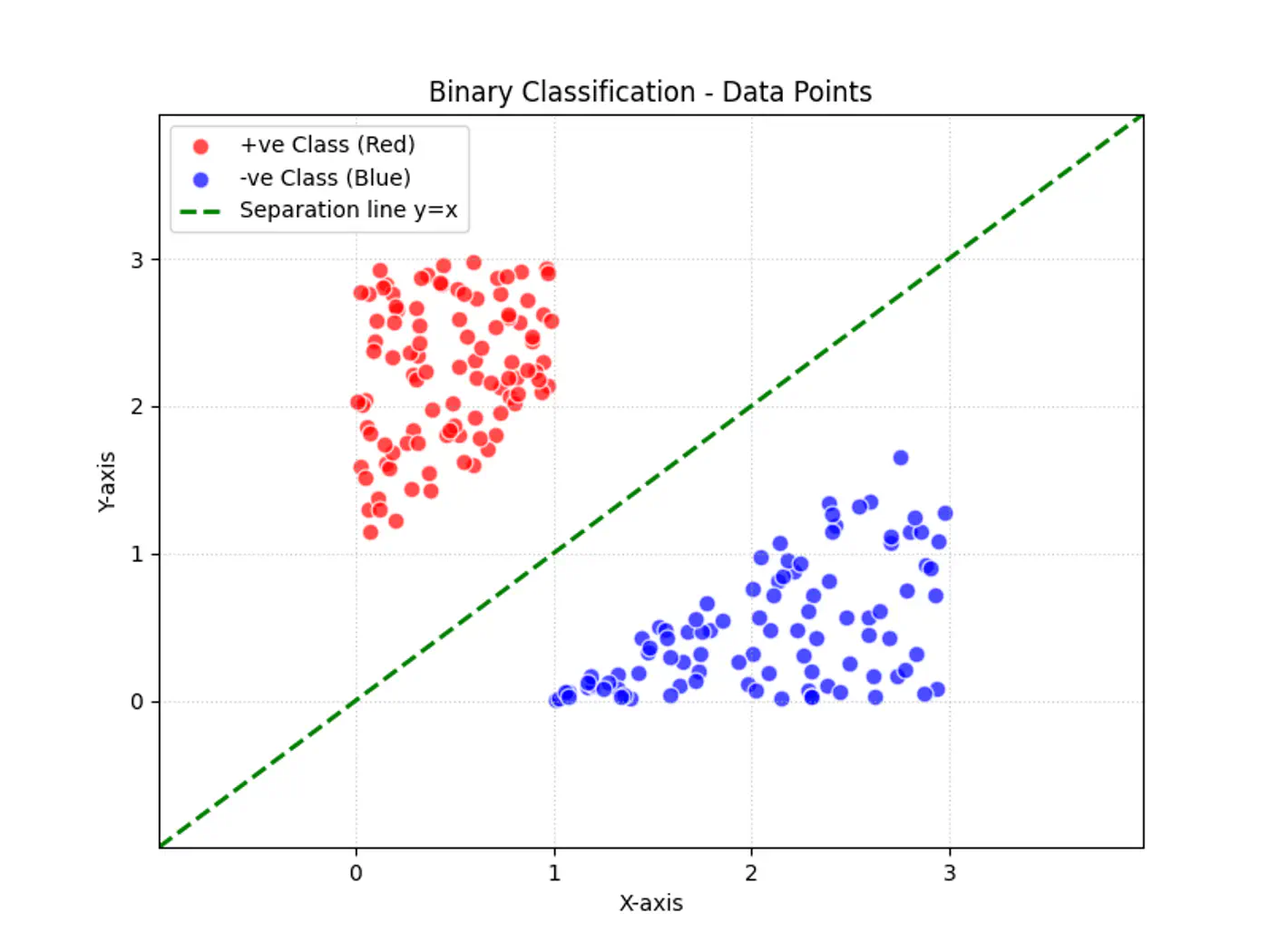
Linear regression tries to find the best fit line, but we want to find the line or decision boundary that clearly separates the two classes.
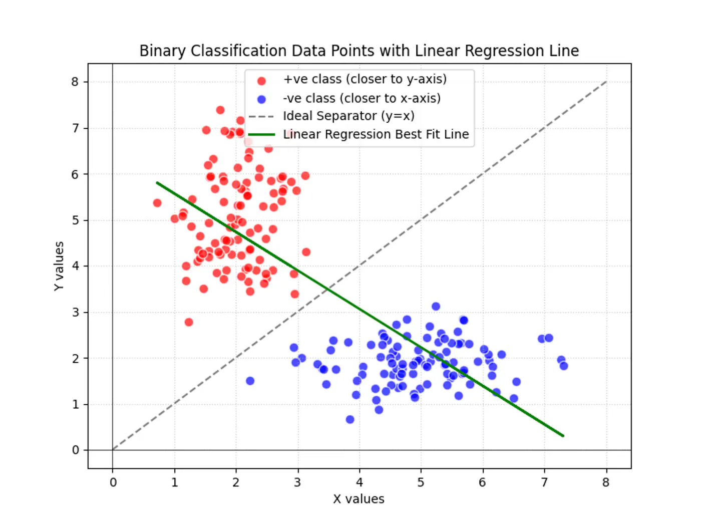
Find the decision boundary, i.e, the equation of the separating hyperplane.
\[z=w^{T}x+w_{0}\]Value of \(z = \mathbf{w^Tx} + w_0\) tells us how far is the point from the decision boundary and on which side.
Note: Weight 🏋️♀️ vector ‘w’ is normal/perpendicular to the hyperplane, pointing towards the positive class (y=1).
- For points exactly on the decision boundary \[z = \mathbf{w^Tx} + w_0 = 0 \]
- Positive (+ve) labeled points \[ z = \mathbf{w^Tx} + w_0 > 0 \]
- Negative (-ve) labeled points \[ z = \mathbf{w^Tx} + w_0 < 0 \]
So we need a link 🔗 to transform the geometric distance to probability.
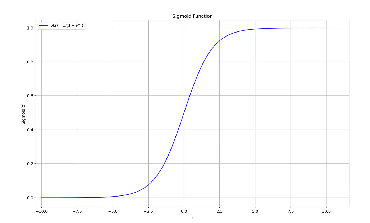
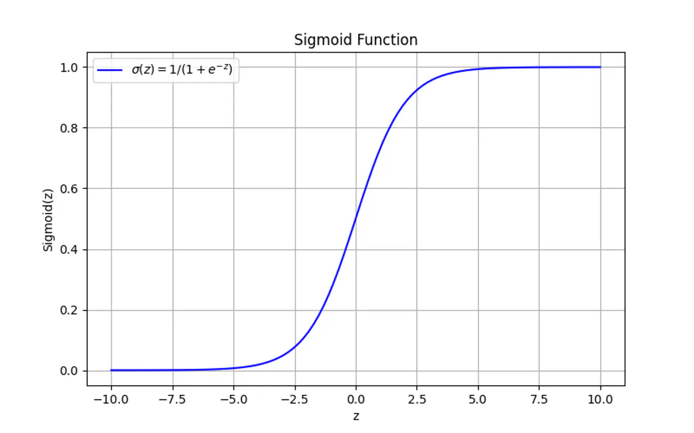
Maps the output of a linear equation to a value between 0 and 1, allowing the result to be interpreted as a probability.
\[\hat{y} = \sigma(z) = \frac{1}{1 + e^{-z}}\]If the distance ‘z’ is large and positive, \(\hat{y} \approx 1\) (High confidence).
If the distance ‘z’ is 0, \(\hat{y} = 0.5\) (Maximum uncertainty).
End of Section
2.2 - Log Loss
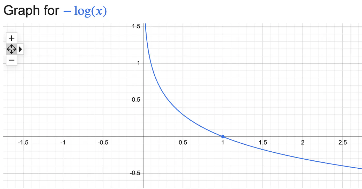
Log Loss = \(\begin{cases} -log(\hat{y_i}) & \text{if } y_i = 1 \\ \\ -log(1-\hat{y_i}) & \text{if } y_i = 0 \end{cases} \)
Combining the above 2 conditions into 1 equation gives:
Log Loss = \(-[y_ilog(\hat{y_i}) + (1-y_i)log(1-\hat{y_i})]\)
We need to find the weights 🏋️♀️ ‘w’ that minimize the cost 💵 function.
- Weight update: \[w_{new}=w_{old}-η.\frac{∂J(w)}{∂w_{old}}\]
We need to find the gradient of log loss w.r.t weight ‘w’.
Chain Rule:
\[\frac{\partial{J(w)}}{\partial{w}} = \frac{\partial{J(w)}}{\partial{\hat{y}}}.\frac{\partial{\hat{y}}}{\partial{z}}.\frac{\partial{z}}{\partial{w}}\]- Cost Function: \(J(w) = -\frac{1}{n}\sum [y_ilog(\hat{y_i}) + (1-y_i)log(1-\hat{y_i})]\)
- Prediction: \(\hat{y} = \sigma(z) = \frac{1}{1 + e^{-z}}\)
- Distance of Point: \(z = \mathbf{w^Tx} + w_0\)
How loss changes w.r.t prediction ?
\[ \begin{align*} \frac{\partial{J(w)}}{\partial{\hat{y}}} &= - [\frac{y}{\hat{y}} - \frac{1-y}{1-\hat{y}}] \\ &= -[\frac{y- \cancel{y\hat{y}} -\hat{y} + \cancel{y\hat{y}}}{\hat{y}(1-\hat{y})}] \\ \therefore \frac{\partial{J(w)}}{\partial{\hat{y}}} &= \frac{\hat{y} - y}{\hat{y}(1-\hat{y})} \end{align*} \]How prediction changes w.r.t distance ?
\[ \begin{align*} \frac{\partial{\hat{y}}}{\partial{z}} &= \frac{\partial{\sigma(z)}}{\partial{z}} = \sigma'(z) \\ \sigma'(z) &= \sigma(z)(1-\sigma(z)) \\ \therefore \frac{\partial{\hat{y}}}{\partial{z}} &= \hat{y}(1-\hat{y}) \end{align*} \]from equations (1) & (2):
\[ \begin{align*} \because \frac{\partial{\sigma(z)}}{\partial{z}} &= \frac{\partial{\sigma(z)}}{\partial{u}}. \frac{\partial{u}}{\partial{z}} \\ \implies \frac{\partial{\sigma(z)}}{\partial{z}} &= - \frac{1}{(1 + e^{-z})^2}. -e^{-z} = \frac{e^{-z}}{(1 + e^{-z})^2} \\ 1 - \sigma(z) & = 1 - \frac{1}{1 + e^{-z}} = \frac{e^{-z}}{1 + e^{-z}} \\ \frac{\partial{\sigma(z)}}{\partial{z}} &= \frac{1}{1 + e^{-z}}.\frac{e^{-z}}{1 + e^{-z}} \\ \therefore \frac{\partial{\sigma(z)}}{\partial{z}} &= \sigma(z).(1-\sigma(z)) \end{align*} \]How distance changes w.r.t weight 🏋️♀️ ?
\[ \frac{\partial{z}}{\partial{w}} = \mathbf{x} \]\[\because \frac{\partial{(a^T\mathbf{x})}}{\partial{\mathbf{x}}} = a\]Chain Rule:
\[ \begin{align*} \frac{\partial{J(w)}}{\partial{w}} &= \frac{\partial{J(w)}}{\partial{\hat{y}}}.\frac{\partial{\hat{y}}}{\partial{z}}.\frac{\partial{z}}{\partial{w}} \\ &= \frac{\hat{y} - y}{\cancel{\hat{y}(1-\hat{y})}}.\cancel{\hat{y}(1-\hat{y})}.x \\ \therefore \frac{\partial{J(w)}}{\partial{w}} &= (\hat{y} - y).x \end{align*} \]Gradient = Error x Input
- Error = \((\hat{y_i}-y_i)\): how far is prediction from the truth?
- Input = \(x_i\): contribution of specific feature to the error.
Weight update:
\[w_{new} = w_{old} - \eta. \sum_{i=1}^n (\hat{y_i} - y_i).x_i\]Mean Squared Error (MSE) can not be used to quantify error/loss in binary classification because:
- Convexity : MSE combined with Sigmoid is non-convex, so, Gradient Descent can get trapped in local minima.
- Penalty: MSE does not appropriately penalize mis-classifications in binary classification.
- e.g: If actual value is class 1 but the model predicts class 0, then MSE = \((1-0)^2 = 1\), which is very low, whereas log loss = \(-log(0) = \infty\)
End of Section
2.3 - Regularization
The weights 🏋️♀️ will tend towards infinity, preventing a stable solution.
The model tries to make probabilities exactly 0 or 1, but the sigmoid function never reaches these limits, leading to extreme weights 🏋️♀️ to push probabilities near the extremes.
Distance of Point: \(z = \mathbf{w^Tx} + w_0\)
Prediction: \(\hat{y} = \sigma(z) = \frac{1}{1 + e^{-z}}\)
Log loss: \(-[y_ilog(\hat{y_i}) + (1-y_i)log(1-\hat{y_i})] \)
Model becomes perfectly accurate on training 🏃♂️data but fails to generalize, performing poorly on unseen data.
Adds a penalty term to the loss function, discouraging weights 🏋️♀️ from becoming too large.
End of Section
2.4 - Log Odds
Odds compare the likelihood of an event happening vs. not happening.
Odds = \(\frac{p}{1-p}\)
- p = probability of success
In logistic regression we assume that Log-Odds (the log of the ratio of positive class to negative class) is a linear function of inputs.
Log-Odds (Logit) = \(log_e \frac{p}{1-p}\)
Log Odds = \(log_e \frac{p}{1-p} = z\)
\[z=w^{T}x+w_{0}\]\[ \begin{align*} &log_{e}(\frac{p}{1-p}) = z \\ &⟹\frac{p}{1-p} = e^{z} \\ &\implies p = e^z - p.e^z \\ &\implies p = \frac{e^z}{1+e^z} \\ &\text { divide numerator and denominator by } e^z \\ &\implies p = \frac{1}{1+e^{-z}} \quad \text { i.e, Sigmoid function} \end{align*} \]- Probability: 0 to 1
- Odds: 0 to + \(\infty\)
- Log Odds: -\(\infty\) to +\(\infty\)
End of Section
2.5 - Probabilistic Interpretation
We assume that our target variable ‘y’ follows a Bernoulli distribution, i.e, has exactly 2 outputs success/failure.
- P(Y=1|X) = p
- P(Y=0|X) = 1- p
Combining above 2 into 1 equation gives:
- P(Y=y|X) = \(p^y(1-p)^{1-y}\)
‘Find the most plausible explanation for what I see.’
We want to find the weights 🏋️♀️‘w’ that maximize the likelihood of seeing the data.
- Data, D = \(\{ (x_i, y_i)_{i=1}^n , \quad y_i \in \{0,1\} \}\)
We do this by maximizing likelihood function.
Assumption: Training data is I.I.D.
A common simplification is to maximize the log-likelihood function instead, which converts the product into a sum.
Note: Log is a strictly monotonically increasing function.
Maximizing the log-likelihood is same as minimizing the negative of log-likelihood.
\[ \begin{align*} \underset{w}{\mathrm{max}}\ log\mathcal{L}(w) &= \underset{w}{\mathrm{min}} - log\mathcal{L}(w) \\ \underset{w}{\mathrm{min}} - log\mathcal{L}(w) &= - \sum_{i=1}^n [ y_ilog(p_i) + (1-y_i)log(1-p_i)] \\ \underset{w}{\mathrm{min}} - log\mathcal{L}(w) &= \text {Log Loss} \end{align*} \]End of Section
3.1 - KNN Introduction
- Parametric models:
- Rely on assumption that relationships between data points are linear.
- For polynomial regression we need to find the degree of polynomial.
- Training:
- We need to train 🏃♂️the model for prediction.
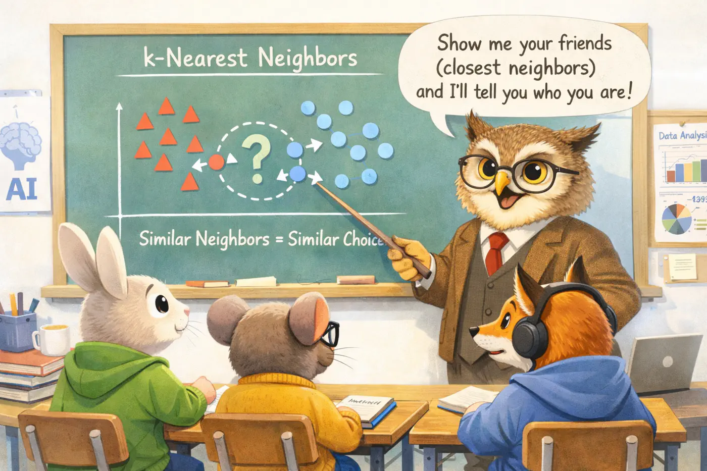
Simple: Intuitive way to classify data or predict values by finding similar existing data points (neighbors).
Non-Parametric: Makes no assumptions about the underlying data distribution.
No Training Required: KNN is a ‘lazy learner’, it does not require a formal training 🏃♂️ phase.

Given a query point \(x_q\) and a dataset, D = {\((x_i,y_i)_{i=1}^n, \quad x_i,y_i \in \mathbb{R}^d\)}, the algorithm finds a set of ‘k’ nearest neighbors \(\mathcal{N}_k(x_q) \subseteq D\).
Inference:
- Choose a value of ‘k’ (hyper-parameter); odd number.
- Calculate distance (Euclidean, Cosine etc.) between and every point in dataset and store in a distance list.
- Sort the distance list in ascending order; choose top ‘k’ data points.
- Make prediction:
- Classification: Take majority vote of ‘k’ nearest neighbors and assign label.
- Regression: Take the mean/median of ‘k’ nearest neighbors.
Note: Store entire dataset.
- Storing Data: Space Complexity: O(nd)
- Inference: Time Complexity ⏰: O(nd + nlogn)
Explanation:
- Distance to all ’n’ points in ‘d’ dimensions: O(nd)
- Sorting all ’n’ data points : O(nlogn)
Note: Brute force 🔨 KNN is unacceptable when ’n’ is very large, say billions.
End of Section
3.2 - KNN Optimizations
Naive KNN needs some improvements to fix some of its drawbacks.
- Standardization
- Distance-Weighted KNN
- Mahalanobis Distance
⭐️Say one feature is ‘Annual Income’ (0-1M), and another feature is ‘Years of Experience’ (0-40).
👉The Euclidean distance will be almost entirely dominated by income 💵.
💡So, we do standardization of each feature, such that it has a mean, \(\mu\)=0 and variance,\(\sigma\)=1.
\[z=\frac{x-\mu}{\sigma}\]⭐️Vanilla KNN treats the 1st nearest neighbor and the k-th nearest neighbor as equal.
💡A neighbor that is 0.1units away should have more influence than a neighbor that is 10 units away.
👉We assign weight 🏋️♀️ to each neighbor; most common strategy is inverse of squared distance.
\[w_i = \frac{1}{d(x_q, x_i)^2 + \epsilon}\]Improvements:
- Noise/Outlier: Reduces the impact of ‘noise’ or ‘outlier’ (distant neighbors).
- Imbalanced Data: Closer points dominate, mitigating impact of imbalanced data.
- e.g: If you have a query point surrounded by 2 very close ‘Class A’ points and 3 distant ‘Class B’ points, weighted 🏋️♀️ KNN will correctly pick ‘Class A'.
⭐️Euclidean distance makes assumption that all the features are independent and provide unique information.
💡‘Height’ and ‘Weight’ are highly correlated.
👉If we use Euclidean distance, we are effectively ‘double-counting’ the size of the person.
🏇Mahalanobis distance measures distance in terms of standard deviations from the mean, accounting for the covariance between features.
\[d(x, y) = \sqrt{(x - y)^T \Sigma^{-1} (x - y)}\]\(\Sigma\): Covariance matrix of the data
- If \(\Sigma\) is identity matrix, Mahalanobis distance reduces to Euclidean distance.
- If \(\Sigma\) is a diagonal matrix, Mahalanobis distance reduces to Normalized Euclidean distance.
🦀Naive KNN shifts all computation 💻 to inference time ⏰, and it is very slow.
- To find the neighbor for one query, we must touch every single bit of the ‘nxd’ matrix.
- If n=10^9,a single query would take seconds, but we need milliseconds.
- Distance Weighted KNN
- K-D Trees (d<20): Recursively partitions space into axis-aligned hyper-rectangles. O(log N ) search.
- Ball Trees : High dimensional data; Haversine distance for geospatial 🌎 data.
- Approximate Nearest Neighbors (ANN)
- Locality Sensitive Hashing (LSH): Uses ‘bucketizing’ 🗑️ hashes. Points that are close have a high probability of having the same hash.
- Hierarchical Navigable Small World (HNSW); Graph of vectors; Search is a ‘greedy walk’ across levels.
- Product Quantization (Reduce memory 🧠 footprint 👣 of high dimensional vectors)
- ScaNN (Google)
- FAISS (Meta)
- Dimensionality Reduction (Mitigate ‘Curse of Dimensionality’)
- PCA
End of Section
3.3 - Curse Of Dimensionality
While Euclidean distance(L norm) is the most frequently discussed, ‘Curse of Dimensionality’ impacts all Minkowski norms (\(L_p\))
\[L_p = (\sum |x_i|^p)^{\frac{1}{p}} \]Note: ‘Curse of Dimensionality’ is largely a function of the exponent (p) in the distance calculation.
Coined 🪙 by mathematician John Bellman in the 1960s while studying dynamic programming.
High dimensional data created following challenges:
- Distance Concentration
- Data Sparsity
- Exponential Sample Requirement
💡Consider a hypercube in d-dimensions of side length = 1; Volume = \(1^d\) = 1
🧊 A smaller inner cube with side length = 1 - \(\epsilon\) ; Volume = \((1 -\epsilon)^d\)
🧐 This implies that almost all the volume of the high-dimensional cube lies near the ‘crust’.
👉e.g: if \(\epsilon\)= 0.01, d = 500; Volume of inner cube = \((1 -0.01)^{500}\) = \(0.99^{500}\) = 0.006 = 0.6%
🤔Consequently, all points become nearly equidistant, and the concept of ‘nearest’ or ‘neighborhood’ loses
its meaning.
⭐️The volume of the feature space increases exponentially with each added dimension.
👉To maintain the same data density found in a 1D space with 10 points, we would need \(10^{10}\)(10 billion) points in 10D space.
💡Because real-world datasets are rarely this large, the data becomes “sparse,” making it difficult to find truly similar neighbors.
⭐️To maintain a reliable result, the amount of training data needed must grow exponentially with the number of dimensions.
👉Without this growth, the model is highly prone to overfitting, where it learns from noise in the ‘sparse’ data rather than actual underlying patterns.
Note: For modern embeddings (often 768 or 1536 dimensions), it is mathematically impossible to collect enough data to ‘fill’ the space.
- Cosine Similarity
- Normalization
Cosine similarity measures the cosine of the angle between 2 vectors.
\[\text{cos}(\theta) = \frac{A \cdot B}{\|A\|\|B\|} = \frac{\sum_{i=1}^{D} A_i B_i}{\sqrt{\sum_{i=1}^{D} A_i^2} \sqrt{\sum_{i=1}^{D} B_i^2}}\]Note: Cosine similarity mitigates the ‘curse of dimensionality" problem.
⭐️Normalize the vector, i.e, make its length =1, a unit vector.
💡By normalizing, we project all points onto the surface of a unit hypersphere.
- We are no longer searching in the ‘empty’ high-dimensional volume of a hypercube.
- Now, we are searching on a constrained manifold (the shell).
Note: By normalizing, we move the data from the volume of the D-dimensional space onto the surface of a (D-1)-dimensional hypersphere.
Euclidean Distance Squared of Normalized Vectors:
\[ \begin{align*} \|A - B\|^2 &= (A - B) \cdot (A - B) \\ &= \|A\|^2 + \|B\|^2 - 2(A \cdot B)\\ \because \|A\| &= \|B\| = 1 \\ \|A - B\|^2 &= 1 + 1 - 2\cos(\theta) \\ \therefore \|A - B\|^2 &= 2(1 - \cos(\theta))\\ \end{align*} \]Note: This formula proves that maximizing ‘Cosine similarity’ is identical to minimizing ‘Euclidean distance’ on the hypersphere.
End of Section
3.4 - Bias Variance Tradeoff
Let’s use this dataset to understand the impact of number of neighbours ‘k’.
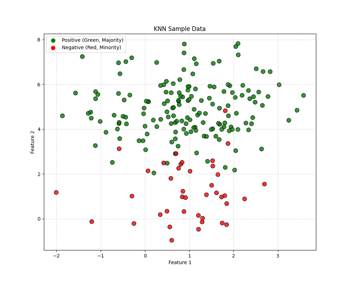
👉If ‘k’ is very large, say, k=n,
- model simply predicts the majority class of the entire dataset for every query point , i.e, under-fitting.
👉If ‘k’ is very small, say, k=1,
- model is highly sensitive to noise or outliers, as it looks at only 1 nearest neighbor, i.e, over-fitting.
Let’s plot Error vs ‘K’ neighbors:
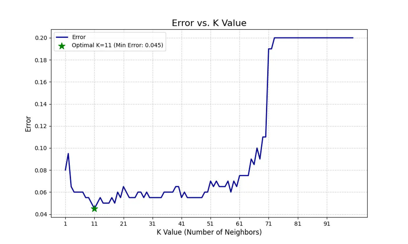
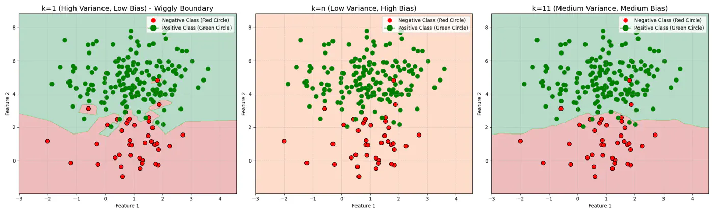
Figure 1: k=1, Over-fitting
Figure 2: k=n, Under-fitting
Figure 3: k=11, Lowest Error (Optimum)
End of Section
4.1 - Decision Trees Introduction
💡It can be written as nested 🕸️ if else statements.
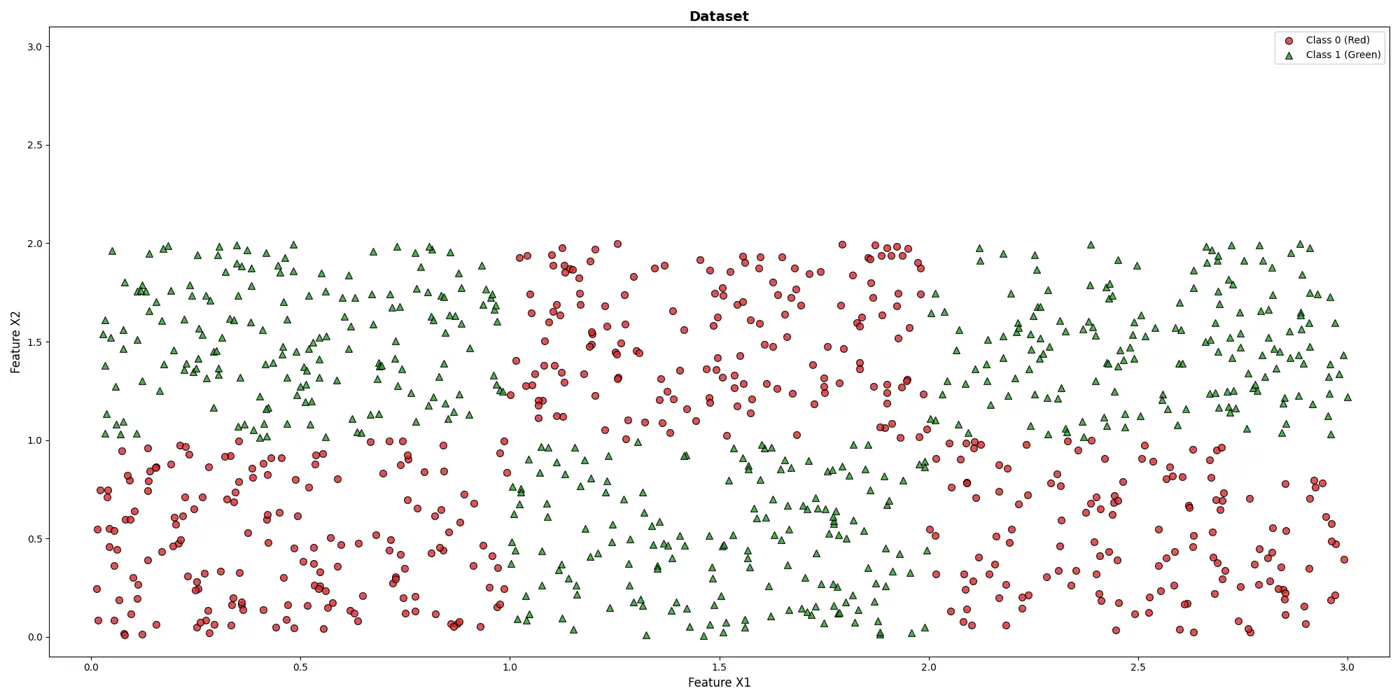
e.g: To classify the left bottom corner red points we can write:
👉if (FeatureX1 <1 & FeatureX2 <1)
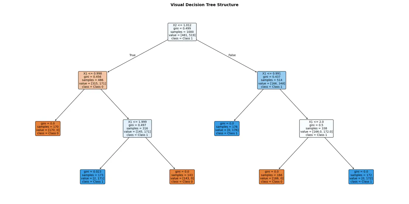
⭐️Extending the logic for all, we have an if else ladder like below:

👉Final decision boundaries will be something like below:
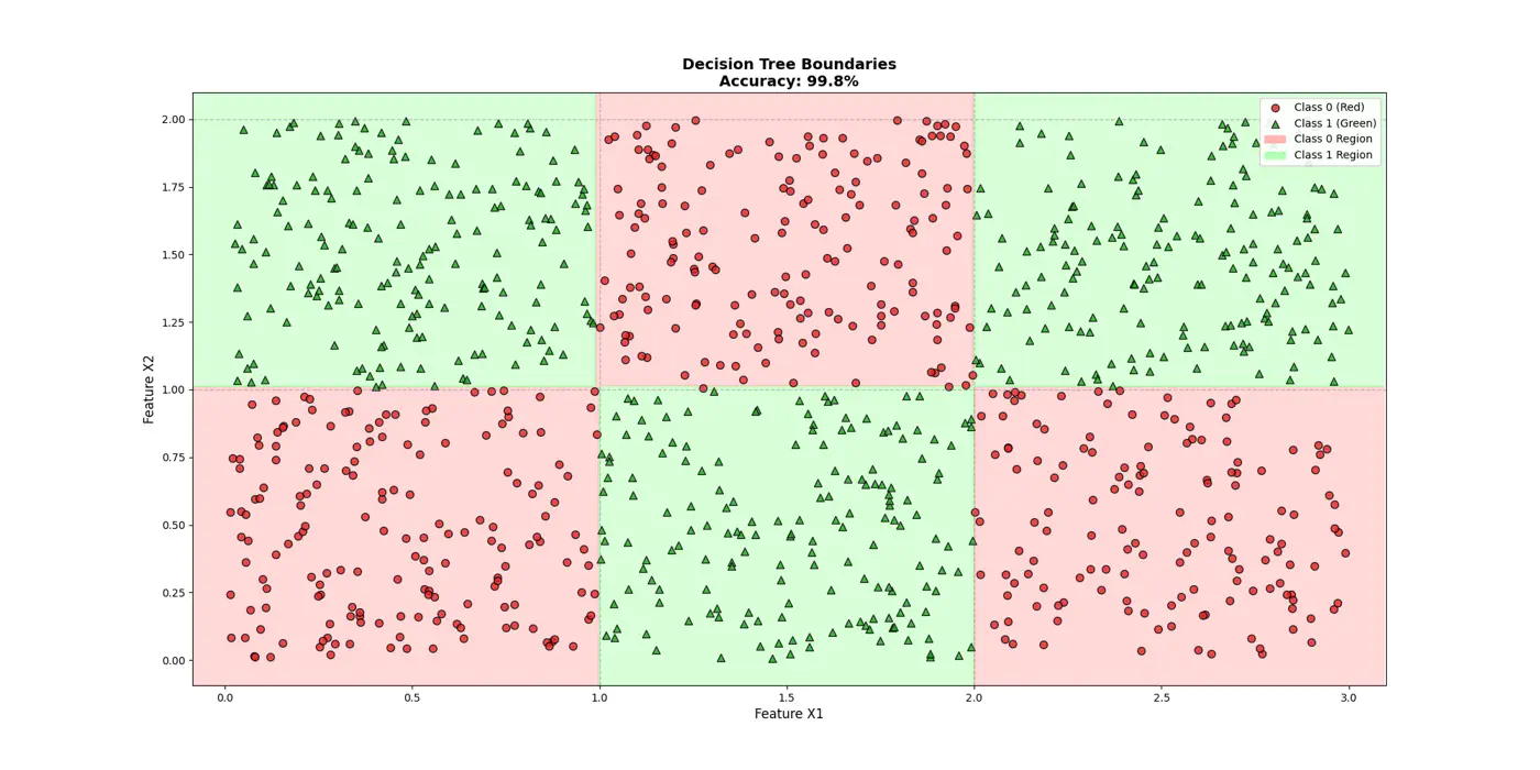
- Non-parametric model.
- Recursively partitions the feature space.
- Top-down, greedy approach to iteratively select feature splits.
- Maximize purity of a node, based on metrics, such as, Information Gain 💵 or Gini 🧞♂️Impurity.
Note: We can extract the if/else logic of the decision tree and write in C++/Java for better performance.
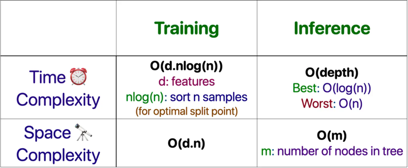
⭐️Building an optimal decision tree 🌲 is a NP-Hard problem.
👉(Time Complexity: Exponential; combinatorial search space)
- Pros
- No standardization of data needed.
- Highly interpretable.
- Good runtime performance.
- Works for both classification & regression.
- Cons
- Number of dimensions should not be too large. (Curse of dimensionality)
- Overfitting.
- As base learners in ensembles, such as, bagging(RF), boosting(GBDT), stacking, cascading, etc.
- As a baseline, interpretable, model or for quick feature selection.
- Runtime performance is important.
End of Section
4.2 - Purity Metrics
Decision trees recursively partition the data based on feature values.
Pure Leaf 🍃 Node: Terminal node where every single data point belongs to the same class.
💡Zero Uncertainty.
The goal of a decision tree algorithm is to find the split that maximizes information gain, meaning it removes the most uncertainty from the data.
So, what is information gain ?
How do we reduce uncertainty ?
Let’s understand few terms first, before we understand information gain.
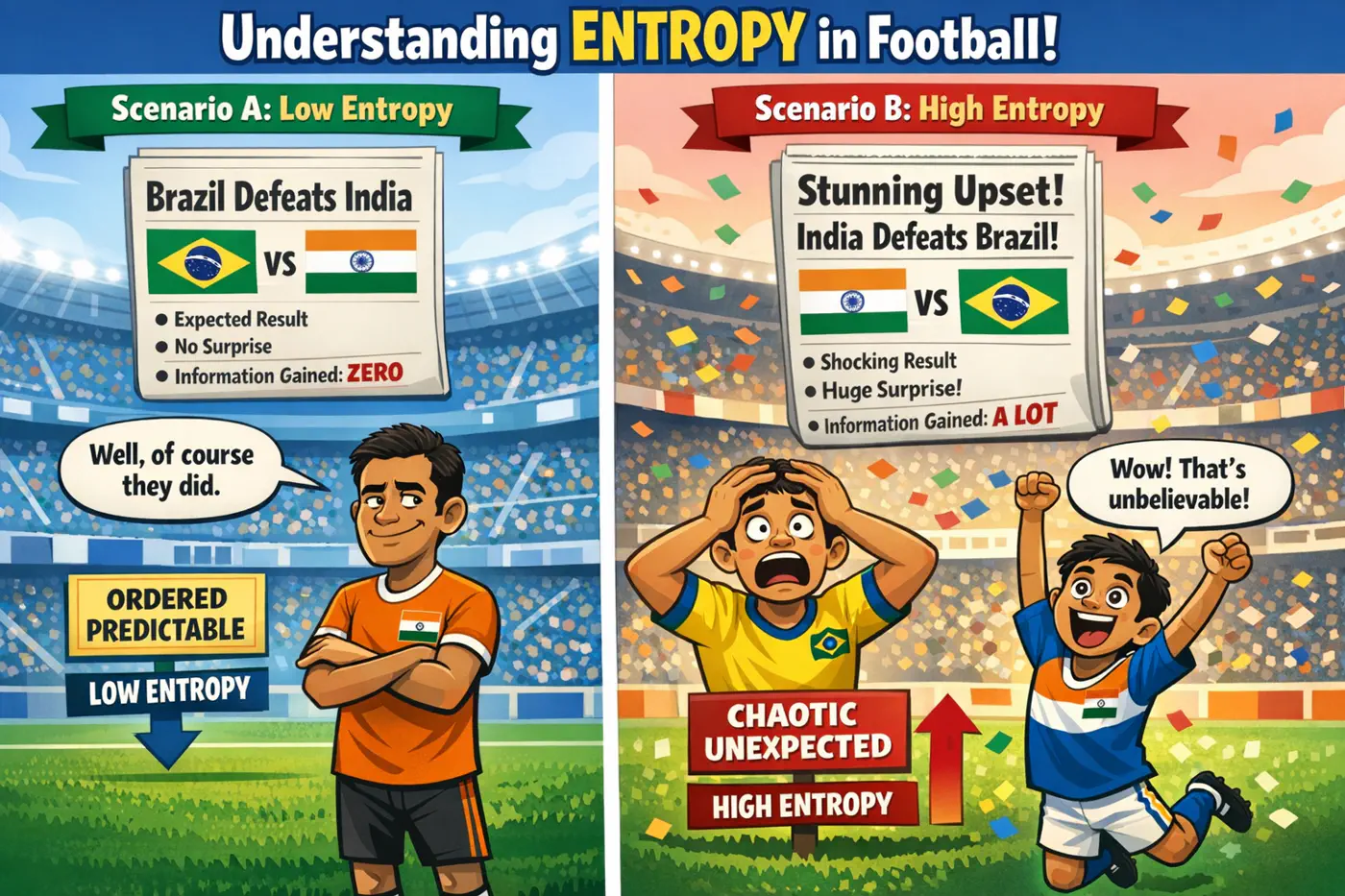
Measure ⏱ of uncertainty, randomness, or impurity in a data.
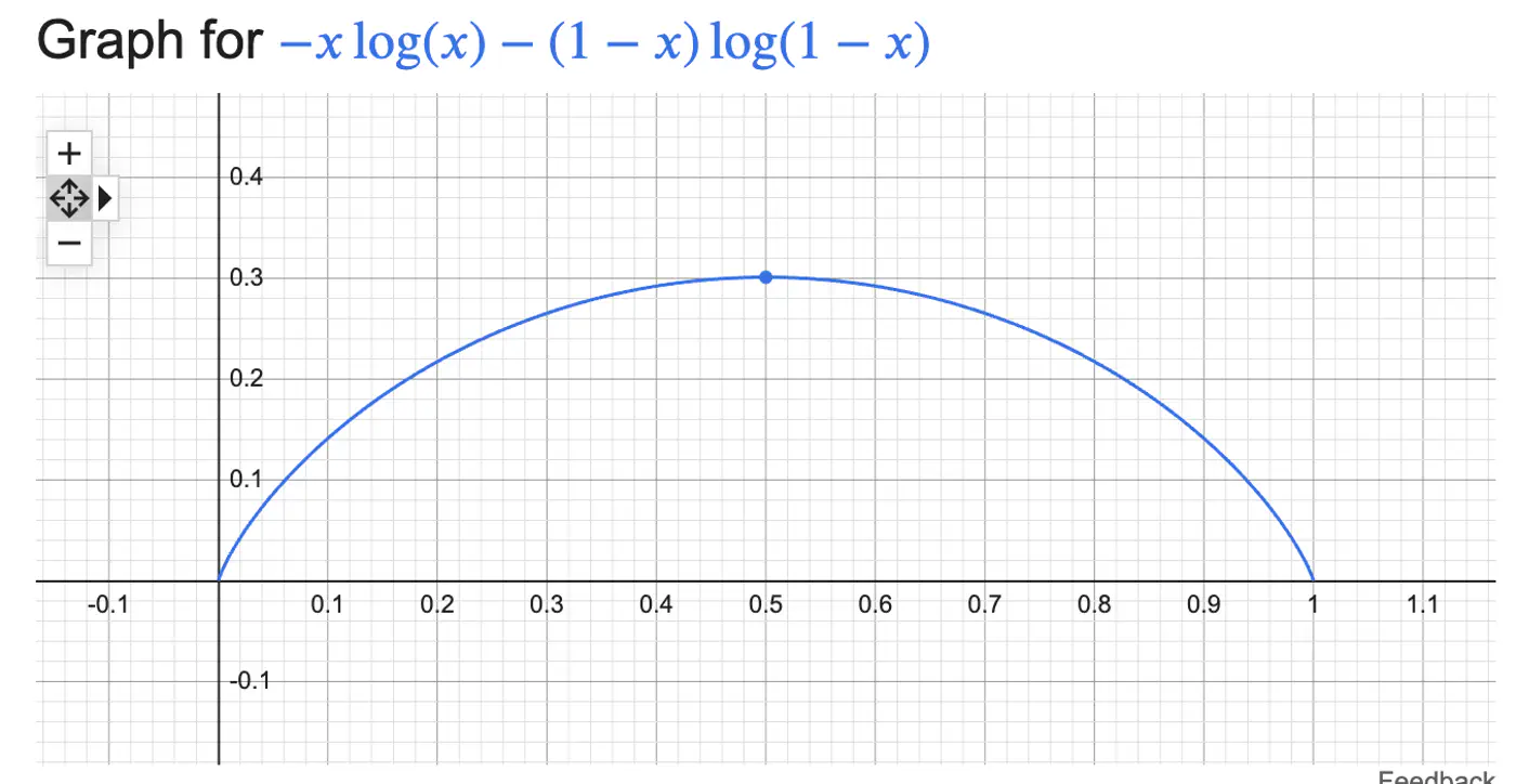
\[H(S)=-\sum _{i=1}^{n}p_{i}\log(p_{i})\]Binary Entropy:
💡Entropy can also be viewed as the ‘average surprise'.
A highly certain event provides little information when it occurs (low surprise).
An unlikely event provides a lot of information (high surprise).
⭐️ Measures the reduction in entropy (uncertainty) achieved by splitting a dataset based on a specific attribute.
\[IG=Entropy(Parent)-\left[\frac{N_{left}}{N_{parent}}Entropy(Child_{left})+\frac{N_{right}}{N_{parent}}Entropy(Child_{right})\right] \]Note: The goal of a decision tree algorithm is to find the split that maximizes information gain, meaning it removes the most uncertainty from the data.
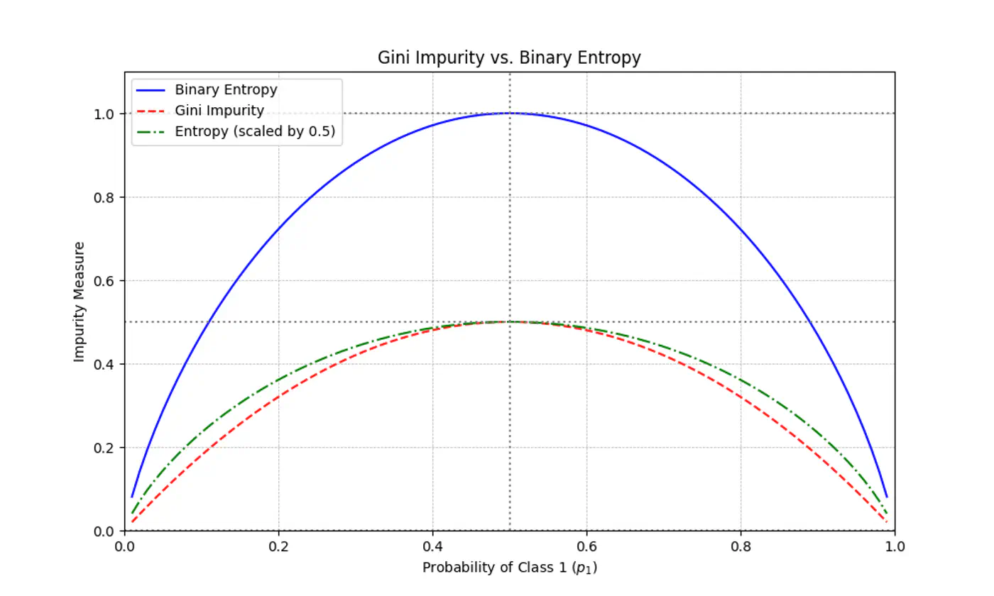
⭐️ Measures the probability of an element being incorrectly classified if it were randomly labeled according to the distribution of labels in a node.
\[Gini(S)=1-\sum_{i=1}^{n}(p_{i})^{2}\]- Range: 0 (Pure) - 0.5 (Maximum impurity)
Note: Gini is used in libraries like Scikit-Learn (as the default), because it avoids the computationally expensive 💰 log function.
Gini Impurity is a first-order approximation of Entropy.
For most of the real-world cases, choosing one over the other results in the exact same tree structure or negligible differences in accuracy.
When we plot the two functions, they follow nearly identical shapes.
End of Section
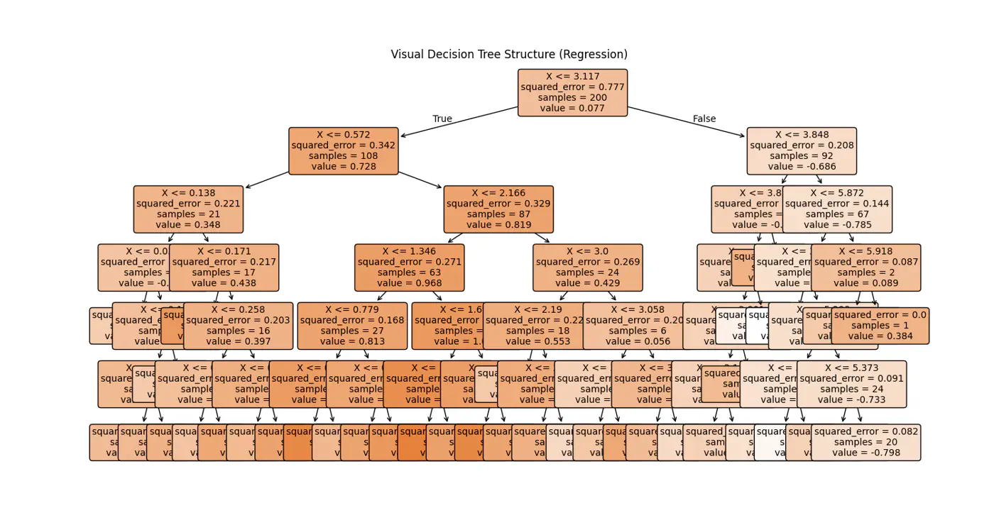
4.3 - Decision Trees For Regression
Decision Trees can also be used for Regression tasks but using a different metrics.
⭐️Metric:
- Mean Squared Error (MSE)
- Mean Absolute Error (MAE)
👉Say we have a following dataset, that we need to fit using decision trees:
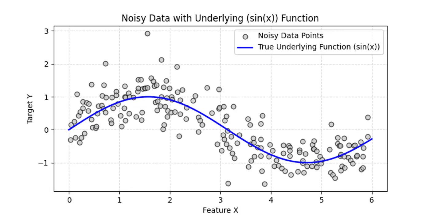
👉Decision trees try to find the decision splits, building step functions that approximate the actual curve, as shown below:
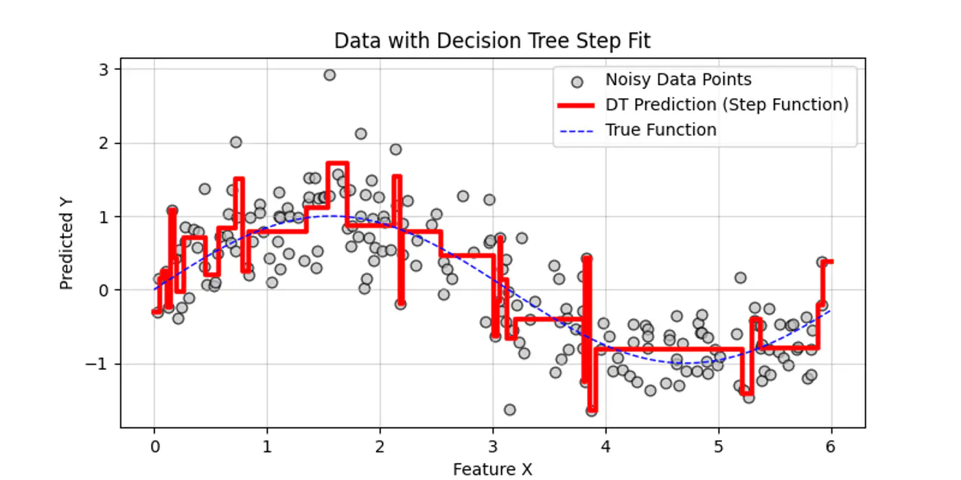
👉Internally the decision tree (if else ladder) looks like below:
Decision trees cannot predict values outside the range of the training data, i.e, extrapolation.
Let’s understand the interpolation and extrapolation cases one by one.
⭐️Predicting values within the range of features and targets observed during training 🏃♂️.
- Trees capture discontinuities perfectly, because they are piece-wise constant.
- They do not try to force a smooth line where a ‘jump’ exists in reality.
e.g: Predicting a house 🏡 price 💰 for a 3-BHK home when you have seen 2-BHK and 4-BHK homes in that same neighborhood.
⭐️Predicting values outside the range of training 🏃♂️data.
Problem:
Because a tree outputs the mean of training 🏃♂️ samples in a leaf, it cannot predict a value higher than the
highest ‘y’ it saw during training 🏃♂️.
- Flat-Line: Once a feature ‘X’ goes beyond the training boundaries, the tree falls into the same ‘last’ leaf forever.
e.g: Predicting the price 💰 of a house 🏡 in 2026 based on data from 2010 to 2025.
End of Section
4.4 - Regularization
- Pre-Pruning ✂️ &
- Post-Pruning ✂️
⭐️ ‘Early stopping’ heuristics (hyper-parameters).
- max_depth: Limits how many levels of ‘if else’ the tree can have; most common.
- min_samples_split: A node will only split, if it has at least ‘N’ samples; smooths the model (especially in regression), by ensuring predictions are based on an average of multiple points.
- max_leaf_nodes: Limiting the number of leaves reduces the overall complexity of the tree, making it simpler and less likely to memorize the training data’s noise.
- min_impurity_decrease: A split is only made if it reduces the impurity (Gini/MSE) by at least a certain threshold.
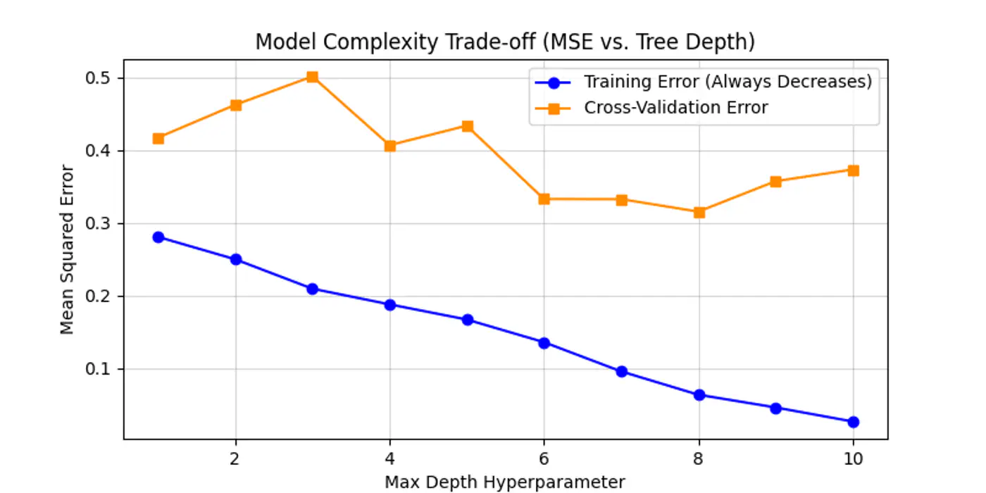
Below is an example for one of the hyper-parameter’s max_depth tuning.
As we can see below the cross-validation error decreases till depth=6 and after that reduction in error is not so significant.
Let the tree🌲 grow to its full depth (overfit) and then ‘collapse’ nodes that provide little predictive value.
Most common algorithm:
- Minimal Cost Complexity Pruning
💡Define a cost-complexity 💰 measure that penalizes the tree 🌲 for having too many leaves 🍃.
\[R_\alpha(T) = R(T) + \alpha |T|\]- R(T): total misclassification rate (or MSE) of the tree
- |T|: number of terminal nodes (leaves)
- \(\alpha\): complexity parameter (the ‘tax’ 💰 on complexity)
Logic:
- If \(\alpha\)=0, the tree is the original overfit tree.
- As \(\alpha\) increases 📈, the penalty for having many leaves grows 📈.
- To minimize the total cost 💰, the model is forced to prune branches that do not significantly reduce R(T).
- Use cross-validation to find the ‘sweet spot’ \(\alpha\) that minimizes validation error.
End of Section
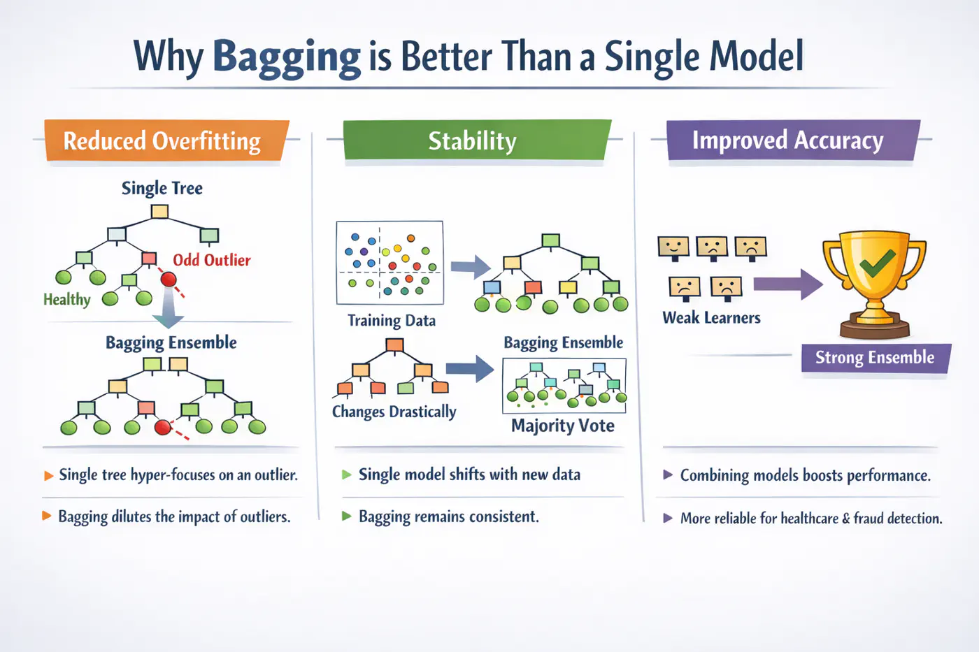
4.5 - Bagging
A single decision tree is highly sensitive to the specific training dataset.
Small changes, such as, a few different rows or the presence of an outlier, can lead to a completely different tree structure.Unpruned decision trees often grow until they perfectly classify the training set, essentially ‘memorizing’ noise and outliers, i.e, high variance, rather than finding general patterns.
Bagging = ‘Bootstrapped Aggregation’
Bagging 🎒is a parallel ensemble technique that reduces variance (without significantly increasing the bias) by training multiple versions of the same model on different random subsets of data and then combining their results.
Note: Bagging uses deep trees (overfit) and combines them to reduce variance.
Bootstrapping = ‘Without external help’
Given a training 🏃♂️set D of size ’n’, we create B new training sets D by sampling ’n’ observations from D ‘with replacement'.
💡Since, we are sampling ‘with replacement’, so, some data points may be picked multiple times, while others may not be picked at all.
- The probability that a specific observation is not selected in a bootstrap sample of size ’n’ is: \[\lim_{n \to \infty} \left(1 - \frac{1}{n}\right)^n = \frac{1}{e} \approx 0.368\]
🧐This means each tree is trained on roughly 63.2% of the unique data, while the remaining 36.8% (the Out-of-Bag or OOB set) can be used for cross validation.
⭐️Say we train ‘B’ models (base-learners), each with variance \(\sigma^2\) .
👉Average variance of ‘B’ models (trees) if all are independent:
\[Var(X)=\frac{\sigma^{2}}{B}\]👉Since, bootstrap samples are derived from the same dataset, the trees are correlated with some correlation coefficient ‘\(\rho\)'.
So, the true variance of bagged ensemble is:
\[Var(f_{bag}) = \rho \sigma^2 + \frac{1-\rho}{B} \sigma^2\]- \(\rho\)= 0; independent models, most reduction in variance.
- \(\rho\)= 1; fully correlated models, no improvement in variance.
- 0<\(\rho\)<1; As correlation decreases, variance reduces .
End of Section
4.6 - Random Forest
💡If one feature is extremely predictive (e.g., ‘Area’ for house prices), almost every bootstrap tree will split on that feature at the root.
👉This makes the trees(models) very similar, leading to a high correlation ‘\(\rho\)’.
\[Var(f_{bagging})=ρ\sigma^{2}+\frac{1-ρ}{B}\sigma^{2}\]💡Choose a random subset of ‘m’ features from the total ‘d’ features, reducing the correlation ‘\(\rho\)’ between trees.
👉By forcing trees to split on ‘sub-optimal’ features, we intentionally increase the variance of individual trees; also the bias is slightly increased (simpler trees).
Standard heuristics:
- Classification: \(m = \sqrt{d}\)
- Regression: \(m = \frac{d}{3}\)
💡Because ‘\(\rho\)’ is the dominant factor in the variance of the ensemble when B is large, the overall ensemble variance Var(\(f_{rf}\)) drops significantly lower than standard Bagging.
\[Var(f_{rf})=ρ\sigma^{2}+\frac{1-ρ}{B}\sigma^{2}\]💡A Random Forest will never overfit by adding more trees (B).
It only converges to the limit: ‘\(\rho\sigma^2\)’.
Overfitting is controlled by:
- depth of the individual trees.
- size of the feature subset ‘m'.
- High Dimensionality: 100s or 1000s of features; RF’s feature sampling prevents a few features from masking others.
- Tabular Data (with Complex Interactions): Captures non-linear relationships without needing manual feature engineering.
- Noisy Datasets: The averaging process makes RF robust to outliers (especially if using min_samples_leaf).
- Automatic Validation: Need a quick estimate of generalization error without doing 10-fold CV (via OOB Error).
End of Section
4.7 - Extra Trees
💡In a standard Decision Tree or Random Forest, the algorithm searches for the optimal split point (the threshold ’s’) that maximizes Information Gain or minimizes MSE.
👉This search is:
- computationally expensive (sort + mid-point) and
- tends to follow the noise in the training 🏃♂️data.
Adding randomness (right kind) in ensemble averaging reduces correlation/variance.
\[Var(f_{bag})=ρ\sigma^{2}+\frac{1-ρ}{B}\sigma^{2}\]- Random Thresholds: Instead of searching for the best split point (computationally expensive 💰) for a feature, it picks a threshold at random from a uniform distribution between the feature’s local minimum and maximum.
- Entire Dataset: Uses entire training dataset (default) for every tree; no bootstrapping.
- Random Feature Subsets: Random subset of m<n features is used in each decision tree.
Picking thresholds randomly has two effects:
- Structural correlation between trees becomes extremely low.
- Individual trees are ‘weaker’ and have higher bias than a standard optimized tree.
👉The massive drop in ‘\(\rho\)’ often outweighs the slight increase in bias, leading to an overall ensemble that is smoother and more robust to noise than a standard Random Forest.
Note: Extra Trees are almost always grown to full depth, as they may need extra splits to find the same decision boundary.
- Performance: Significantly faster to train, as it does not sort data to find optimal split.
Note: If we are working with billions of rows or thousands of features, ET can be 3x to 5x faster than a Random Forest(RF). - Robustness to Noise: By picking thresholds randomly, tends to ‘handle’ the noise more effectively than RF.
- Feature Importance: Because ET is so randomized, it often provides more ‘stable’ feature importance scores.
Note: It is less likely to favor a high-cardinality feature (e.g. zip-code) just because it has more potential split points.
End of Section
4.8 - Boosting
⭐️In Bagging 🎒we trained multiple strong(over-fit, high variance) models (in parallel) and then averaged them out to reduce variance.
💡Similarly, we can train many weak(under-fit, high bias) models sequentially, such that, each new model corrects the errors of the previous ones to reduce bias.
⚔️ An ensemble learning approach where multiple ‘weak learners’ (typically simple models like shallow decision trees 🌲 or ‘stumps’) are sequentially combined to create a single strong predictive model.
⭐️The core principle is that each subsequent model focuses 🎧 on correcting the errors made by its predecessors.
- AdaBoost(Adaptive Boosting)
- Gradient Boosting Machine (GBM)
- XGBoost
- LightGBM (Microsoft)
- CatBoost (Yandex)
End of Section
4.9 - AdaBoost
💡Works by increasing 📈 the weight 🏋️♀️ of misclassified data points after each iteration, forcing the next weak learner to ‘pay more attention’🚨 to the difficult cases.
⭐️ Commonly used for classification.
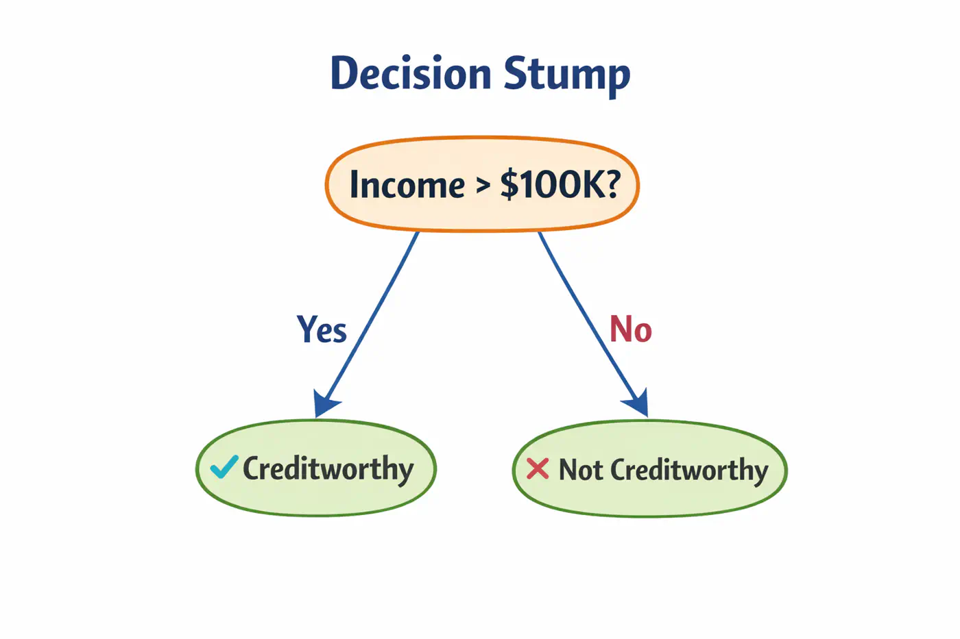
👉Weak learners are typically ‘Decision Stumps’, i.e, decision trees🌲with a depth of only one (1 split, 2 leaves 🍃).
- Assign an equal weight 🏋️♀️to every data point; \(w_i = 1/n\), where ’n’=number of samples.
- Build a decision stump that minimizes the weighted classification error.
- Calculate total error; \(E_m = \Sigma w_i\).
- Determine ‘amount of say’, i.e, the weight 🏋️♀️ of each stump in final decision.
\[\alpha_m = \frac{1}{2}ln\left( \frac{1-E_m}{E_m} \right)\]
- Low error results in a high positive \(\alpha\) (high influence).
- 50% error (random guessing) results in an \(\alpha = 0\) (no influence).
- Update sample weights 🏋️♀️.
- Misclassified samples: Weight 🏋️♀️ increases by \(e^{\alpha_m}\).
- Correctly classified samples: Weight 🏋️♀️ decreases by \(e^{-\alpha_m}\).
- Normalization: All new weights 🏋️♀️ are divided by their total sum so they add up back to 1.
- Iterate for a specified number of estimators (n_estimators).
👉 To classify a new data point, every stump makes a prediction (+1 or -1).
These are multiplied by their respective ‘amount of say’ \(\alpha_m\) and summed.
\[H(x)=sign\sum_{m=1}^{M}\alpha_{m}⋅h_{m}(x)\]👉 If the total weighted 🏋️♀️ sum is positive, the final class is +1; otherwise -1.
Note: Sensitive to outliers; Because AdaBoost aggressively increases weights 🏋️♀️ on misclassified points, it may ‘over-focus’ on noisy outliers, hurting performance.
End of Section
4.10 - Gradient Boosting Machine
GBM treats the final model \(F_m(x)\) as weighted 🏋️♀️ sum of ‘m’ weak learners:
\[ F_{M}(x)=\underbrace{F_{0}(x)}_{\text{Initial\ Guess}}+\nu \sum _{m=1}^{M}\underbrace{\left(\sum _{j=1}^{J_{m}}\gamma _{jm}\mathbb{I}(x\in R_{jm})\right)}_{\text{Weak\ Learner\ }h_{m}(x)}\]- \(F_0(x)\): The initial base model (usually a constant).
- M: The total number of boosting iterations (number of trees).
- \(\gamma_{jm}\)(Leaf Weight): The optimized value for leaf in tree .
- \(\nu\)(Nu): The Learning Rate or Shrinkage; prevent overfitting.
- \(\mathbb{I}(x\in R_{jm})\): ‘Indicator Function’; It is 1 if data point falls into leaf of the tree, and 0 otherwise.
- \(R_{jm}\)(Regions): Region of \(j_{th}\) leaf in \(m_{th}\)tree.
📍In Gradient Descent, we update parameters ‘\(\Theta\)';
📍In GBM, we update the predictions F(x) themselves.
🦕We move the predictions in the direction of the negative gradient of the loss function L(y, F(x)).
🎯We want to minimize loss:
\[\mathcal{L}(F) = \sum_{i=1}^n L(y_i, F(x_i))\]✅ In parameter optimization we update weights 🏋️♀️:
\[w_{t+1} = w_t - \eta \cdot \nabla_{w}\mathcal{L}(w_t)\]✅ In gradient boosting, we update the prediction function:
\[F_m(x) = F_{m-1}(x) -\eta \cdot \nabla_F \mathcal{L}(F_{m-1}(x))\]➡️ The gradient is calculated w.r.t. predictions, not weights.
In GBM we can use any loss function as long as it is differentiable, such as, MSE, log loss, etc.
Loss(MSE) = \((y_i - F_m(x_i))^2\)
\[\frac{\partial L}{F_m(x_i)} = -2 (y-F_m(x_i))\]\[\implies \frac{\partial L}{F_m(x_i)} \propto - (y-F_m(x_i))\]👉Pseudo Residual (Error) = - Gradient
💡To minimize loss, take derivative of loss function w.r.t ‘\(\gamma\)’ and equate to 0:
\[F_0(x) = \arg\min_{\gamma} \sum_{i=1}^n L(y_i, \gamma)\]MSE Loss = \(\mathcal{L}(y_i, \gamma) = \sum_{i=1}^n(y_i -\gamma)^2\)
\[ \begin{aligned} &\frac{\partial \mathcal{L}(y_i, \gamma)}{\partial \gamma} = -2 \cdot \sum_{i=1}^n(y_i -\gamma) = 0 \\ &\implies \sum_{i=1}^n (y_i -\gamma) = 0 \\ &\implies \sum_{i=1}^n y_i = n.\gamma \\ &\therefore \gamma = \frac{1}{n} \sum_{i=1}^n y_i \end{aligned} \]💡To minimize cost, take derivative of cost function w.r.t ‘\(\gamma\)’ and equate to 0:
Cost Function = \(J(\gamma )\)
\[J(\gamma )=\sum _{x_{i}\in R_{jm}}\frac{1}{2}(y_{i}-(F_{m-1}(x_{i})+\gamma ))^{2}\]We know that:
\[ r_{i}=y_{i}-F_{m-1}(x_{i})\]\[\implies J(\gamma )=\sum _{x_{i}\in R_{jm}}\frac{1}{2}(r_{i}-\gamma )^{2}\]\[\frac{d}{d\gamma }\sum _{x_{i}\in R_{jm}}\frac{1}{2}(r_{i}-\gamma )^{2}=\sum _{x_{i}\in R_{jm}}-(r_{i}-\gamma )=0\]\[\implies \sum _{x_{i}\in R_{jm}}\gamma -\sum _{x_{i}\in R_{jm}}r_{i}=0\]👉Since, \(\gamma\) is constant for all \(n_j\) samples in the leaf, \(\sum _{x_{i}\in R_{jm}}\gamma =n_{j}\gamma \)
\[n_{j}\gamma =\sum _{x_{i}\in R_{jm}}r_{i}\]\[\implies \gamma =\frac{\sum _{x_{i}\in R_{jm}}r_{i}}{n_{j}}\]Therefore, \(\gamma\) = average of all residuals in the leaf.
Note: \(R_{jm}\)(Regions): Region of \(j_{th}\) leaf in \(m_{th}\)tree.
End of Section
4.11 - GBDT Algorithm
Gradient Boosted Decision Tree (GBDT) is a decision tree based implementation of Gradient Boosting Machine (GBM).
GBM treats the final model \(F_m(x)\) as weighted 🏋️♀️ sum of ‘m’ weak learners (decision trees):
\[ F_{M}(x)=\underbrace{F_{0}(x)}_{\text{Initial\ Guess}}+\nu \sum _{m=1}^{M}\underbrace{\left(\sum _{j=1}^{J_{m}}\gamma _{jm}\mathbb{I}(x\in R_{jm})\right)}_{\text{Decision\ Tree\ }h_{m}(x)}\]- \(F_0(x)\): The initial base model (usually a constant).
- M: The total number of boosting iterations (number of trees).
- \(\gamma_{jm}\)(Leaf Weight): The optimized value for leaf in tree .
- \(\nu\)(Nu): The Learning Rate or Shrinkage; prevent overfitting.
- \(\mathbb{I}(x\in R_{jm})\): ‘Indicator Function’; It is 1 if data point falls into leaf of the tree, and 0 otherwise.
- \(R_{jm}\)(Regions): Region of \(j_{th}\) leaf in \(m_{th}\)tree.
- Step 1: Initialization.
- Step 2: Iterative loop 🔁 : for i=1 to m.
- 2.1: Calculate pseudo residuals ‘\(r_{im}\)'.
- 2.2: Fit a regression tree 🌲‘\(h_m(x)\)'.
- 2.3:Compute leaf 🍃weights 🏋️♀️ ‘\(\gamma_{jm}\)'.
- 2.4:Update the model.
Start with a function that minimizes our loss function;
for MSE its mean.
MSE Loss = \(\mathcal{L}(y_i, \gamma) = \sum_{i=1}^n(y_i -\gamma)^2\)
Find the ‘gradient’ of error;
Tells us the direction and magnitude needed to reduce the loss.
Train a tree to predict the residuals ‘\(h_m(x)\)';
- Tree 🌲 partitions the data into leaves 🍃 (\(R_{jm}\)regions )
Within each leaf 🍃, we calculate the optimal value ‘\(\gamma_{jm}\)’ that minimizes the loss for the samples in that leaf 🍃.
\[\gamma_{jm} = \arg\min_{\gamma} \sum_{x_i \in R_{jm}} L(y_i, F_{m-1}(x_i) + \gamma)\]➡️ The optimal leaf 🍃value is the ‘Mean’(MSE) of the residuals; \(\gamma = \frac{\sum r_i}{n_j}\)
Add the new ‘correction’ to the existing model, scaled by the learning rate.
\[F_{m}(x)=F_{m-1}(x)+\nu \cdot \underbrace{\sum _{j=1}^{J_{m}}\gamma _{jm}\mathbb{I}(x\in R_{jm})}_{h_{m}(x)}\]- \(\mathbb{I}(x\in R_{jm})\): ‘Indicator Function’; It is 1 if data point falls into leaf of the tree, and 0 otherwise.
End of Section
4.12 - GBDT Example
Gradient Boosted Decision Tree (GBDT) is a decision tree based implementation of Gradient Boosting Machine (GBM).
GBM treats the final model \(F_m(x)\) as weighted 🏋️♀️ sum of ‘m’ weak learners (decision trees):
\[ F_{M}(x)=\underbrace{F_{0}(x)}_{\text{Initial\ Guess}}+\nu \sum _{m=1}^{M}\underbrace{\left(\sum _{j=1}^{J_{m}}\gamma _{jm}\mathbb{I}(x\in R_{jm})\right)}_{\text{Decision\ Tree\ }h_{m}(x)}\]- \(F_0(x)\): The initial base model (usually a constant).
- M: The total number of boosting iterations (number of trees).
- \(\gamma_{jm}\)(Leaf Weight): The optimized value for leaf in tree .
- \(\nu\)(Nu): The Learning Rate or Shrinkage; prevent overfitting.
- \(\mathbb{I}(x\in R_{jm})\): ‘Indicator Function’; It is 1 if data point falls into leaf of the tree, and 0 otherwise.
- \(R_{jm}\)(Regions): Region of \(j_{th}\) leaf in \(m_{th}\)tree.
- Step 1: Initialization.
- Step 2: Iterative loop 🔁 : for i=1 to m.
- 2.1: Calculate pseudo residuals ‘\(r_{im}\)'.
- 2.2: Fit a regression tree 🌲‘\(h_m(x)\)'.
- 2.3:Compute leaf 🍃weights 🏋️♀️ ‘\(\gamma_{jm}\)'.
- 2.4:Update the model.
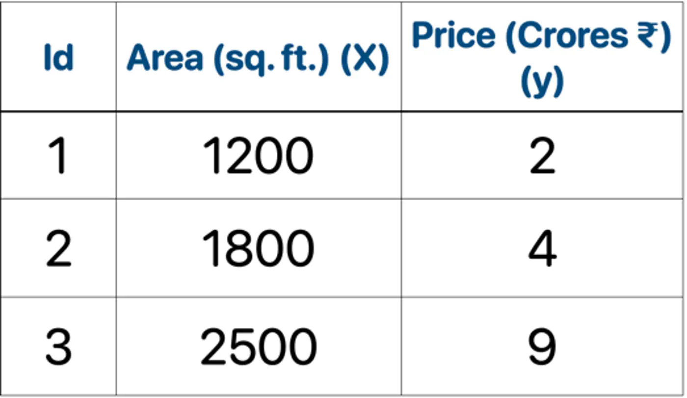
👉Loss = MSE, Learning rate (\(\nu\)) = 0.5
- Initialization : \(F_0(x) = mean(2,4,9) = 5.0\)
- Iteration 1(m=1):
2.1: Calculate residuals ‘\(r_{i1}\)'
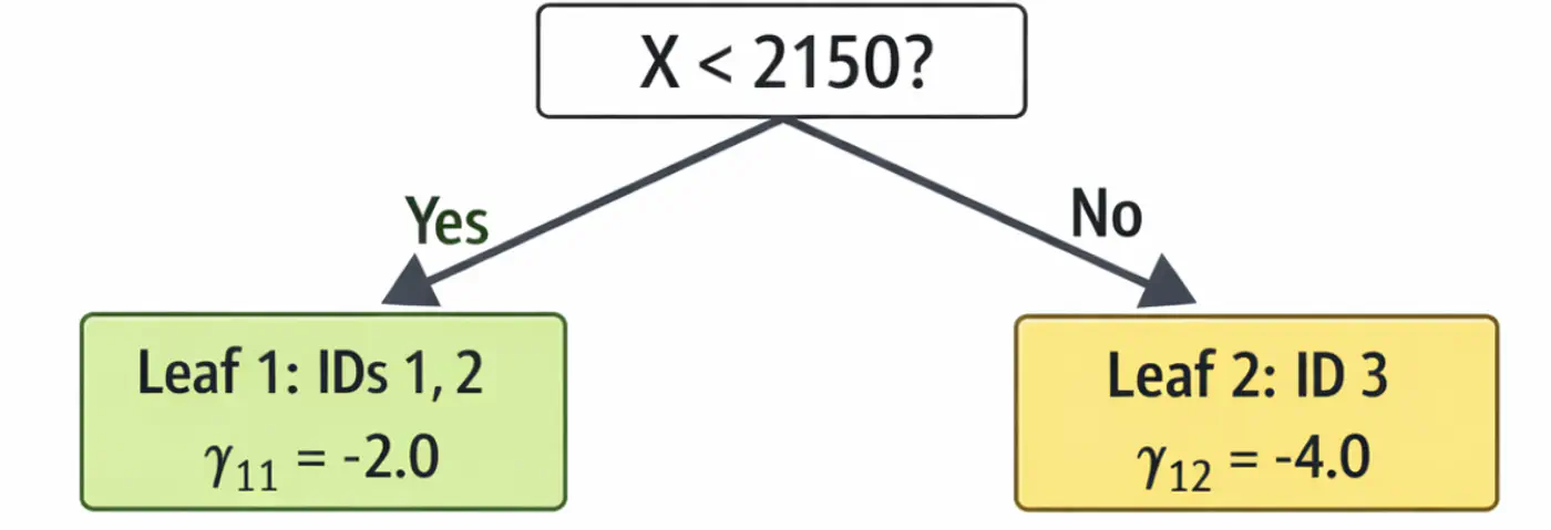
\[\begin{aligned} r_{11} &= 2-5 = -3.0 \\ r_{21} &= 4-5 = -1.0 \\ r_{31} &= 9-5 = 4.0 \\ \end{aligned} \]2.2: Fit tree(\(h_1\)); Split at X<2150 (midpoint of 1800 and 2500)
2.3: Compute leaf weights \(\gamma_{j1}\)
- Y-> Leaf 1: Ids 1, 2 ( \(\gamma_{11}\)= -2.0)
- N-> Leaf 2: Id 3 ( \(\gamma_{21}\)= 4.0)
2.4: Update predictions (\(F_1 = F_0 + 0.5 \cdot \gamma\))
\[ \begin{aligned} F_1(x_1) &= 5.0 + 0.5(-2.0) = \mathbf{4.0}\ \\F_1(x_2) &= 5.0 + 0.5(-2.0) = \mathbf{4.0}\ \\F_1(x_3) &= 5.0 + 0.5(4.0) = \mathbf{7.0}\ \\ \end{aligned} \]Tree 1:
- Iteration 2(m=2):
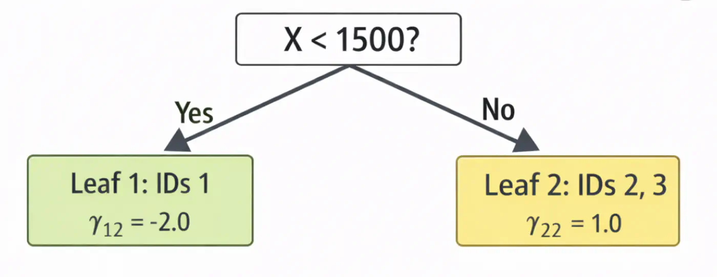
2.1: Calculate residuals ‘\(r_{i2}\)'
\[ \begin{aligned} r_{12} &= 2-4.0 = -2.0 \\ r_{22} &= 4-4.0 = 0.0 \\ r_{32} &= 9-7.0 = 2.0 \\ \end{aligned} \]2.2: Fit tree(\(h_2\)); Split at X<1500 (midpoint of 1200 and 1800)
2.3: Compute leaf weights \(\gamma_{j2}\)
- Y-> Leaf 1: Ids 1 ( \(\gamma_{12}\)= -2.0)
- N-> Leaf 2: Id 2, 3 ( \(\gamma_{22}\)= 1.0)
2.4: Update predictions (\(F_1 = F_0 + 0.5 \cdot \gamma\))
\[ \begin{aligned} F_2(x_1) &= 4.0 + 0.5(-2.0) = \mathbf{3.0} \\F_2(x_2) &= 4.0 + 0.5(1.0) = \mathbf{4.5} \\ F_2(x_3) &= 7.0 + 0.5(1.0) = \mathbf{7.5}\ \\ \end{aligned} \]Tree 2:
Note: We can keep adding more trees with every iteration;
ideally, learning rate \(\nu\) is small, say 0.1, so that we do not overshoot and converge slowly.
Let’s predict the price of a house with area = 2000 sq. ft.
- \(F_{0}=5.0\)
- Pass though tree 1 (\(h_1\)): is 2000 < 2150 ? Yes, \(\gamma_{11}\)= -2.0
- Contribution (\(h_1\)) = 0.5 x (-2.0) = -1.0
- Pass though tree 2 (\(h_2\)): is 2000 < 1500 ? No, \(\gamma_{22}\) = 1.0
- Contribution(\(h_2\)) = 0.5 x (1.0) = 0.5
- Final prediction = 5.0 - 1.0 + 0.5 = 4.5
Therefore, the price of a house with area = 2000 sq. ft is Rs 4.5 crores, which is very close.
In just 2 iterations, although with higher learning rate (\(\nu=0.5\)), we were able to get a fairly good estimate.
End of Section
4.13 - Advanced GBDT Algorithms
🔵 LightGBM (Light Gradient Boosting Machine)
⚫️ CatBoost (Categorical Boosting)
⭐️An optimized and highly efficient implementation of gradient boosting.
👉 Widely used in competitive data science (like Kaggle) due to its speed and performance.
Note: Research project developed by Tianqi Chen during his doctoral studies at the University of Washington.
⭐️Developed by Microsoft, this framework is designed for high speed and efficiency with large datasets.
👉It grows trees leaf-wise rather than level-wise and uses Gradient-based One-Side Sampling (GOSS) to speed 🐇 up the finding of optimal split points.
End of Section
4.14 - XgBoost
⭐️An optimized and highly efficient implementation of gradient boosting.
👉 Widely used in competitive data science (like Kaggle) due to its speed and performance.
Note: Research project developed by Tianqi Chen during his doctoral studies at the University of Washington.
🔵 Regularization
🔵 Sparsity-Aware Split Finding
⭐️Uses second derivative (Hessian), i.e, curvature, in addition to first derivative (gradient) to optimize the objective function more quickly and accurately than GBDT.
Let’s understand this with the problem to minimize \(f(x) = x^4\), using:
Gradient descent (uses only 1st order derivative, \(f'(x) = 4x^3\))
Newton’s method (uses both 1st and 2nd order derivatives \(f''(x) = 12x^2\))

- Adds explicit regularization terms (L1/L2 on leaf weights and tree complexity) into the boosting objective, helping reduce over-fitting. \[ \text{Objective} = \underbrace{\sum_{i=1}^{n} L(y_i, \hat{y}_i)}_{\text{Training Loss}} + \underbrace{\gamma T + \frac{1}{2}\lambda \sum_{j=1}^{T} w_j^2 + \alpha \sum_{j=1}^{T} |w_j|}_{\text{Regularization (The Tax)}} \]
💡Real-world data often contains many missing values or zero-entries (sparse data).
👉 XGBoost introduces a ‘default direction’ for each node.
➡️During training, it learns the best direction (left or right) for missing values to go, making it significantly faster and more robust when dealing with sparse or missing data.
End of Section
4.15 - LightGBM
⭐️Developed by Microsoft, this framework is designed for high speed and efficiency with large datasets.
👉It grows trees leaf-wise rather than level-wise and uses Gradient-based One-Side Sampling (GOSS) to speed 🐇 up the finding of optimal split points.
🔵 Exclusive Feature Bundling (EFB)
🔵 Leaf-wise Tree Growth Strategy
- ❌ Traditional GBDT uses all data instances for gradient calculation, which is inefficient.
- ✅ GOSS focuses 🔬on instances with larger gradients (those that are less well-learned or have higher error).
- 🐛 Keeps all instances with large gradients but randomly samples from those with small gradients.
- 🦩This way, it prioritizes the most informative examples for training, significantly reducing the data used and speeding up 🐇 the process while maintaining accuracy.
- 🦀 High-dimensional data often contains many sparse, mutually exclusive features (features that never take a non-zero value simultaneously, such as, One Hot Encoding (OHE)).
- 💡 EFB bundles the non-overlapping features into a single, dense feature, reducing the number of features, without losing much information, saving computation.
- ❌ Traditional gradient boosting machines (like XGBoost), the trees are built level-wise (BFS-like), meaning all nodes at the current level are split before moving to the next level.
- ✅ LightGBM maintains a set of all potential leaves that can be split at any given time and selects the leaf (for splitting) that provides the maximum gain across the entire tree, regardless of its depth.
Note: Need mechanisms to avoid over-fitting.
End of Section
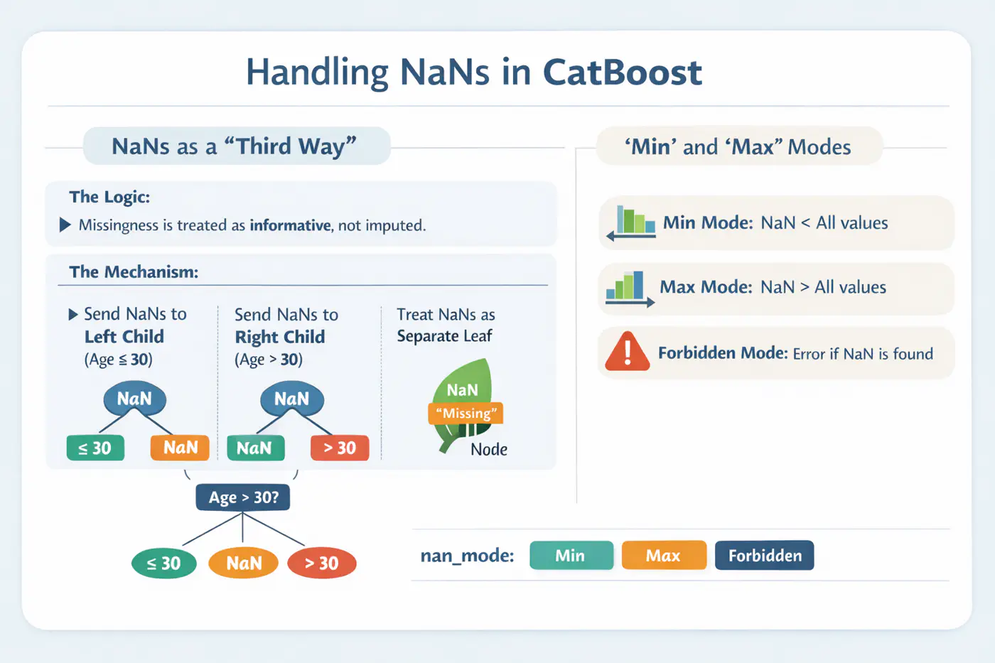
4.16 - CatBoost
🔵 Symmetric(Oblivious) Trees
🔵 Handling Missing Values
- ❌ Standard target encoding can lead to target leakage, where the model uses information from the target variable during training that would not be available during inference.
👉(model ‘cheats’ by using a row’s own label to predict itself). - ✅ CatBoost calculates the target statistics (average target value) for each category based only on the history of previous training examples in a random permutation of the data.
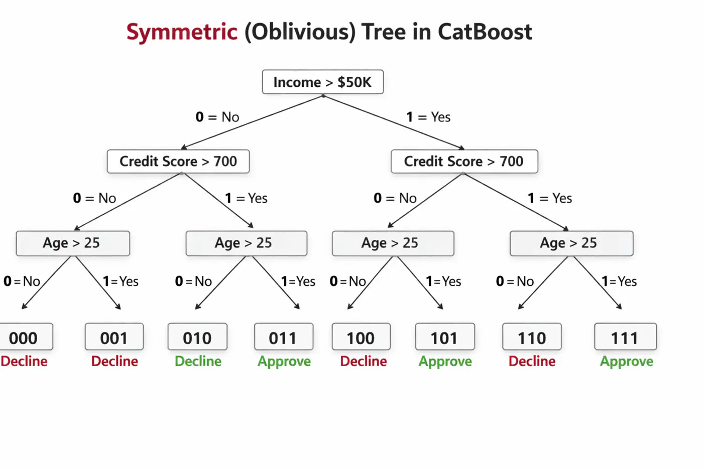
🦋 Uses symmetric decision trees by default.
👉 In symmetric trees, the same split condition is applied at each level across the entire tree structure.🦘Does not walk down the tree using ‘if-else’ logic, instead it evaluates decision conditions to create a binary index (e.g 101) and jumps directly to that leaf 🍃 in memory 🧠.
⚙️ CatBoost offers built-in, intelligent handling of missing values and sparse features, which often require manual preprocessing in other GBDT libraries.
💡Treats ‘NaN’ as a distinct category, reducing the need for imputation.
End of Section
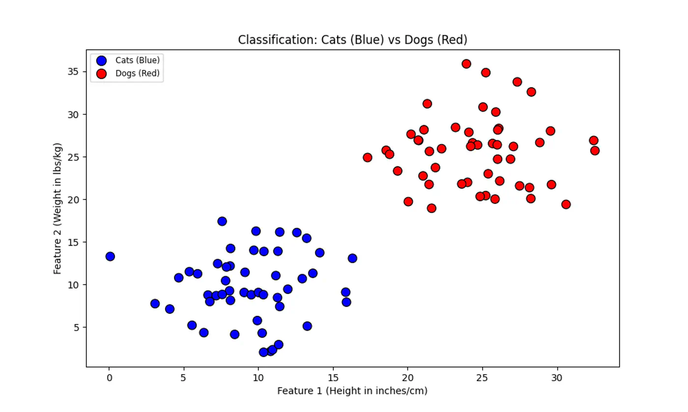
5.1 - SVM Intro
⭐️We have two classes of points (e.g. Cats 😸vs. Dogs 🐶) that can be separated by a straight line.
👉 Many such lines exist !
💡SVM asks: “Which line is the safest?”
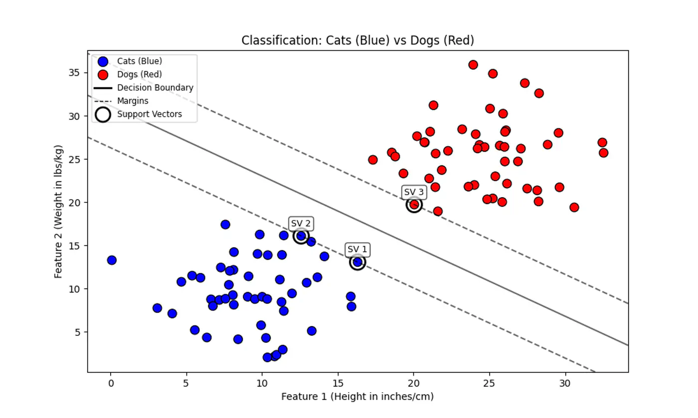
💡Think of the decision boundary as the center-line of a highway 🛣️.
SVM tries to make this highway 🛣️ as wide as possible without hitting any ‘buildings’ 🏡 (data points) on either side.
End of Section
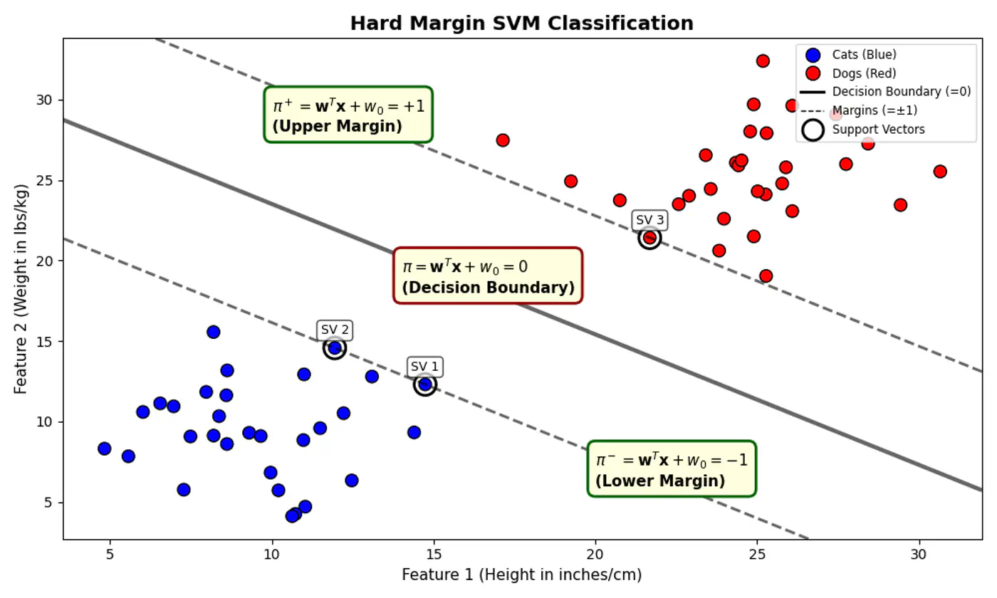
5.2 - Hard Margin SVM
Data is perfectly linearly separable, i.e, there must exist a hyperplane that can perfectly separate the data into two distinct classes without any misclassification.
No noise or outliers that fall within the margin or on the wrong side of the decision boundary. Note: Even a single outlier can prevent the algorithm from finding a valid solution or drastically affect the boundary’s position, leading to poor generalization.
- 🐎 Distance(signed) of a hyperplane from origin = \(\frac{-w_0}{\|w\|}\)
- 🦣 Margin width = distance(\(\pi^+, \pi^-\))
- = \(\frac{1-w_0 - (-1 -w_0)}{\|w\|}\) = \(\frac{1-\cancel{w_0} + 1 + \cancel{w_0})}{\|w\|}\)
- distance(\(\pi^+, \pi^-\)) = \(\frac{2}{\|w\|}\)
Figure: Distance of Hyperplane from Origin
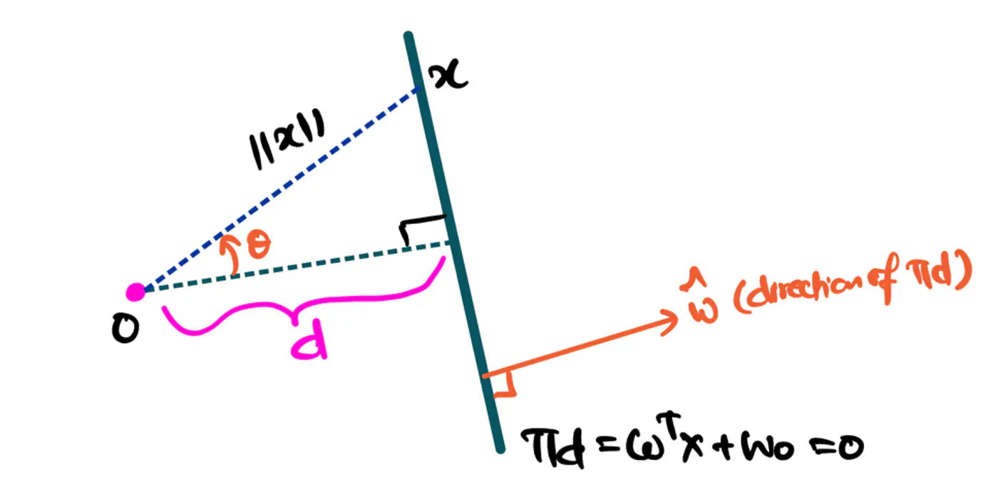
- Separating hyperplane \(\pi\) is exactly equidistant from \(\pi^+\) and \(\pi^-\).
- We want to maximize the margin between +ve(🐶) and -ve (😸) points.
👉Combining above two constraints:
\[y_{i}.(w^{T}x_{i}+w_{0})≥1\]such that, \(y_i.(w^Tx_i + w_0) \ge 1\)
👉To maximize the margin, we must minimize \(\|w\|\).
Since, distance(\(\pi^+, \pi^-\)) = \(\frac{2}{\|w\|}\)
such that, \(y_i.(w^Tx_i + w_0) \ge 1 ~ \forall i = 1,2,\dots, n\)
Note: Hard margin SVM will not work if the data has a single outlier or slight overlap.
End of Section
5.3 - Soft Margin SVM
💡Imagine the margin is a fence 🌉.
Hard Margin: fence is made of steel.
Nothing can cross it.Soft Margin: fence is made of rubber(porous).
Some points can ‘push’ into the margin or even cross over to the wrong side, but we charge them a penalty 💵 for doing so.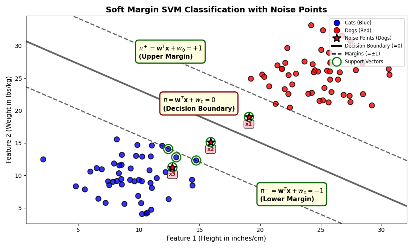
Distance from decision boundary:
- Distance of positive labelled points must be \(\ge 1\)
- But, distance of noise 📢 points (actually positive points) \(x_1, x_2 ~\&~ x_3\) < 1
⚔️ So, we introduce a slack variable or allowance for error term, \(\xi_i\) (pronounced ‘xi’) for every single data point.
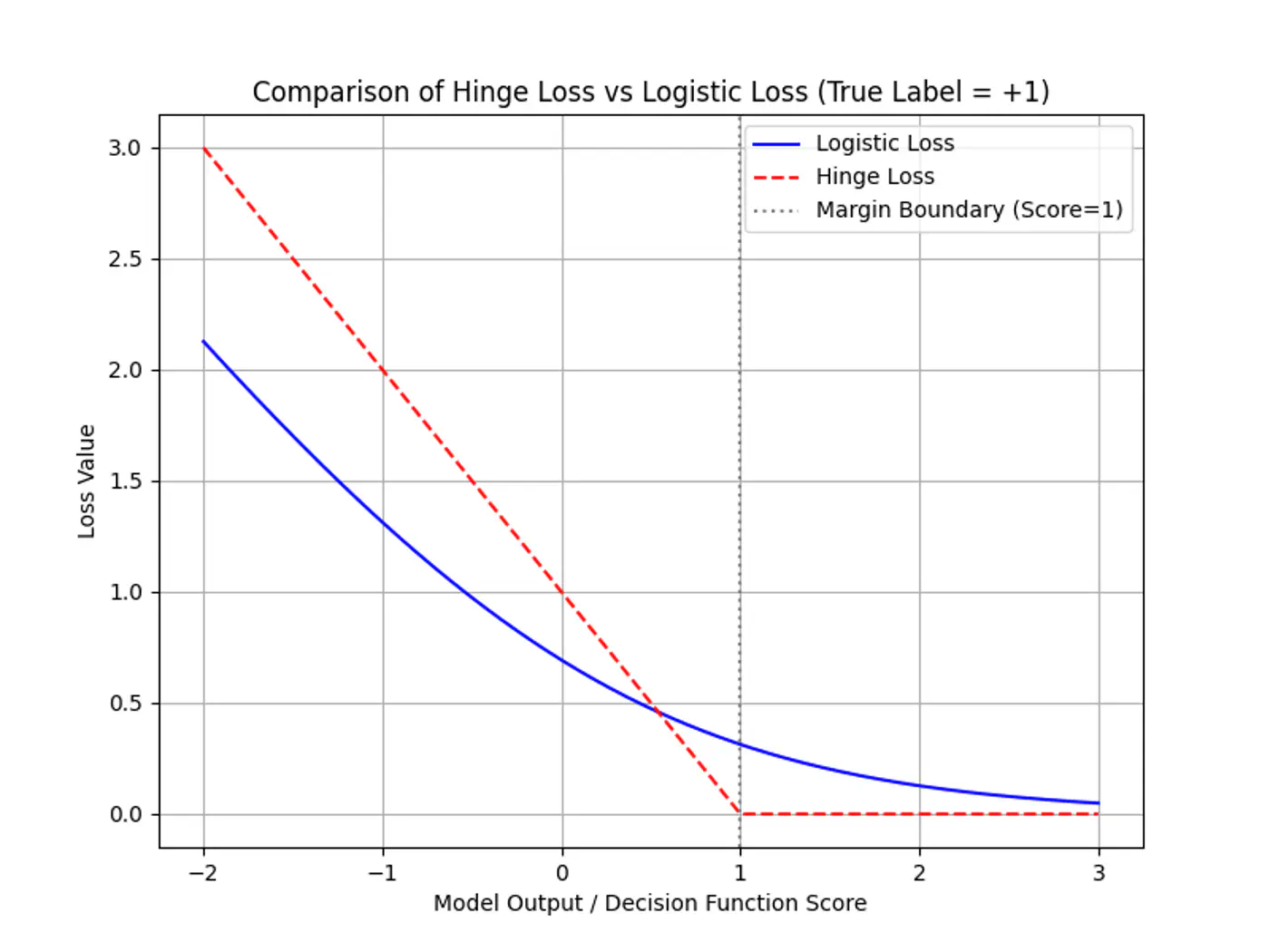
\[y_i.(w^Tx_i + w_0) \ge 1 - \xi_i, ~ \forall i = 1,2,\dots, n\]\[ \implies \xi_i \ge 1 - y_i.(w^Tx_i + w_0) \\ also, ~ \xi_i \ge 0 \]\[So, ~ \xi _{i}=\max (0,1-y_{i}\cdot (w^Tx_i + w_0))\]Note: The above error term is also called ‘Hinge Loss’.
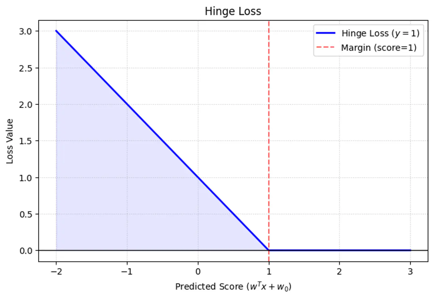
Hinge
- \(\xi_i = 0\) : Correctly classified and outside (or on) the margin.
- \(0 < \xi_i \le 1 \) : Within the margin but on the correct side of the decision boundary.
- \(\xi_i > 0\): On the wrong side of the decision boundary (misclassified).
e.g.: Since, the noise 📢 point are +ve (\(y_i=1\)) labeled:
\[\xi _{i}=\max (0,1-f(x_{i}))\]\(x_1, (d=+0.5)\): \(\xi _{i}=\max (0,1-0.5) = 0.5\)
\(x_2, (d=-0.5)\): \(\xi _{i}=\max (0,1-(-0.5))= 1.5\)
\(x_3, (d=-1.5)\): \(\xi _{i}=\max (0,1-(-1.5)) = 2.5\)

Subject to constraints:
- \(y_i(w^T x_i + b) \geq 1 - \xi_i\): The ‘softened’ margin constraint.
- \(\xi_i \geq 0\): Slack/Error cannot be negative.
Note: We use a hyper-parameter ‘C’ to control the trade-off.
- Large ‘C’: Over-Fitting;
Misclassifications are expensive 💰.
Model tries to keep the errors as low as possible. - Small ‘C’: Under-Fitting;
Margin width is more important than individual errors.
Model will ignore outliers/noise to get a ‘cleaner’(wider) boundary.
Note: SVM is just L2-Regularized Hinge Loss minimization, as Logistic Regression minimizes Log-Loss.
End of Section
5.4 - Primal Dual Equivalence
The Primal form is intuitive but computationally expensive in high dimensions.
➡️ Number of new features = \({d+p \choose p}\), grows roughly as \(O(d^{p})\)
- d= number of dimensions (features)
- p = degree of polynomial
Note: The Dual form is what enables the Kernel Trick 🪄.
Subject to constraints:
- \(y_i(w^T x_i + b) \geq 1 - \xi_i\): The ‘softened’ margin constraint.
- \(\xi_i \geq 0\): Slack/Error cannot be negative.
⭐️ We start with the Soft-Margin Primal objective and incorporate its constraints using Lagrange Multipliers \((\alpha_i, \mu_i \geq 0)\)
\[L(w, w_0, \xi, \alpha, \mu) = \frac{1}{2}\|w\|^2 + C \sum_{i=1}^n \xi_i - \sum_{i=1}^n \alpha_i \left[y_i(w^T x_i + w_0) - 1 + \xi_i \right] - \sum_{i=1}^n \mu_i \xi_i\]Note: Inequality conditions must be \(\le 0\).
👉The Lagrangian function has two competing objectives:
\[L(w, w_0, \xi, \alpha, \mu) = \frac{1}{2}\|w\|^2 + C \sum_{i=1}^n \xi_i - \sum_{i=1}^n \alpha_i \left[y_i(w^T x_i + w_0) - 1 + \xi_i \right] - \sum_{i=1}^n \mu_i \xi_i\]- Minimization: We want to minimize \(L(w, w_0, \xi, \alpha, \mu)\) w.r.t primal variables (\(w, w_0, \xi_i \) ) to find the hyperplane with the largest possible margin.
- Maximization: We want to maximize \(L(w, w_0, \xi, \alpha, \mu)\) w.r.t dual variables (\(\alpha_i, \mu_i\) ) to ensure all training constraints are satisfied.
Note: A point that is simultaneously a minimum for one set of variables and a maximum for another is, by definition, a saddle point.
👉To find the Dual, we find the saddle point by taking partial derivatives with respect to the primal variables \((w, w_0, \xi)\) and equating them to 0.
\[\frac{\partial L}{\partial w} = 0 \implies \mathbf{w = \sum_{i=1}^n \alpha_i y_i x_i}\]\[\frac{\partial L}{\partial w_0} = 0 \implies \mathbf{\sum_{i=1}^n \alpha_i y_i = 0}\]\[\frac{\partial L}{\partial \xi_i} = 0 \implies C - \alpha_i - \mu_i = 0 \implies \mathbf{0 \leq \alpha_i \leq C}\]subject to: \(0 \leq \alpha_i \leq C\) and \(\sum \alpha_i y_i = 0\)
- \(\alpha_i\)= 0, for non support vectors (correct side)
- \(0 < \alpha_i < C\), for free support vectors (exactly on the margin)
- \(\alpha_i = C\), for bounded support vectors (misclassified or inside margin)
Note: Sequential Minimal Optimization (SMO) algorithm is used to find optimal \(\alpha_i\) values.
🎯To classify unseen point \(x_q\) : \(f(x_q) = \text{sign}(w^T x_q + w_0)\)
✅ From the KKT stationarity condition, we know: \(\mathbf{w} = \sum_{i=1}^n \alpha_i y_i x_i\)
👉 Substituting this into the equation:
\[f(x_q) = \text{sign}\left( \sum_{i=1}^n \alpha_i y_i (x_i^T x_q) + w_0 \right)\]Note: Even if you have 1 million training points, if only 500 are support vectors, the summation only runs for 500 terms.
All other points have \(\alpha_i = 0\) and vanish.
End of Section
5.5 - Kernel Trick
👉If our data is not linearly separable in its original space , we can map it to a higher-dimensional feature space (where D»d) using a transformation function .
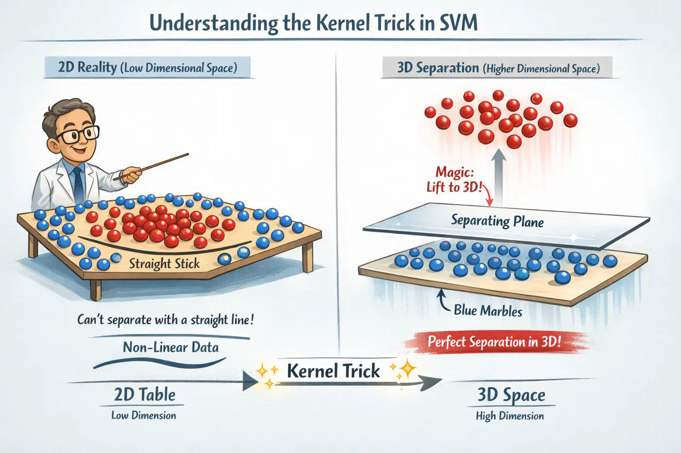
- Bridge between Dual formulation and the geometry of high dimensional spaces.
- It is a way to manipulate inner product spaces without the computational cost 💰 of explicit transformation.
subject to: \(0 \leq \alpha_i \leq C\) and \(\sum \alpha_i y_i = 0\)
💡Actual values of the input vectors \(x_i\) and \(x_j\) never appear in isolation; only appear as inner product.
\[ \max_{\alpha} \sum_{i=1}^n \alpha_i - \frac{1}{2} \sum_{i,j=1}^n \alpha_i \alpha_j y_i y_j \mathbf{(x_i \cdot x_j)}\]\[f(x_q) = \text{sign}\left( \sum_{i=1}^n \alpha_i y_i (x_i^T x_q) + w_0 \right)\]👉The ‘shape’ of the decision boundary is entirely determined by how similar points are to one another, not by their absolute coordinates.
So we define a function called ‘Kernel Function’.
The ‘Kernel Trick’ 🪄 is an optimization that replaces the dot product of a high-dimensional mapping with a function of the dot product in the original space.
\[(x_i, x_j) = \langle \phi(x_i), \phi(x_j) \rangle\]💡How it works ?
Instead of mapping (to higher dimension) \(x_i \rightarrow \phi(x_i)\), \(x_j \rightarrow \phi(x_j)\),
and calculating the dot product.
We simply compute \(K(x_i, x_j)\) directly in the original input space.
👉The ‘Kernel Function’ gives the similar mathematical equivalent of mapping it to a higher dimensions and taking the dot product.
Note: For \(K(x_i, x_j)\) to be a valid kernel, it must satisfy Mercer’s Condition.
Below is an example for a quadratic Kernel function in 2D that is equivalent to mapping the vectors to 3D and taking a dot product in 3D.
\[K(x, z) = (x^T z)^2\]\[(x_1 z_1 + x_2 z_2)^2 = x_1^2 z_1^2 + 2x_1 z_1 x_2 z_2 + x_2^2 z_2^2\]The output of above quadratic kernel function is equivalent to the explicit dot product of two vectors in 3D:
\[\phi(x) = [x_1^2, \sqrt{2}x_1x_2, x_2^2]^T\]\[\phi(z) = [z_1^2, \sqrt{2}z_1z_2, z_2^2]^T\]\[\phi (x)\cdot \phi (z)=x_{1}^{2}z_{1}^{2}+2x_{1}x_{2}z_{1}z_{2}+x_{2}^{2}z_{2}^{2}\]- Computational Efficiency: Avoids the ‘combinatorial blowup’ 💥 of generating thousands of interaction features manually.
- Memory Savings: No need to store 💾 or process high-dimensional coordinates, only the scalar result of the kernel function.
- Designing special purpose domain specific kernel is very hard.
- Basically, we are trying to replace feature engineering with kernel design.
- Note: Deep learning does feature engineering implicitly for us.
- Runtime complexity depends on number of support vectors, whose count is not easy to control.
Note: Runtime Time Complexity ⏰ = \(O(n_{SV}\times d)\) , whereas linear SVM,\(O(d)\) .
End of Section
5.6 - RBF Kernel
- Unlike the polynomial kernel, which looks at global 🌎 interactions, the RBF kernel acts like a similarity measure.
- If ‘x’ and ‘z’ are identical \(K(x,z)=1\).
- As they move further apart in Euclidean space, the value decays exponentially towards 0.
- If \(x \approx z\) (very close), \(K(x,z)=1\)
- If ‘x’, ‘z’ are far apart, \(K(x,z) \approx 0\)
Note: Kernel function is the measure of similarity or closeness.
Say \(\sigma = 1\), then Euclidean distance: \(\|x - z\|^2 = \|x\|^2 + \|z\|^2 - 2x^Tz\)
\[K(x, z) = \exp(-( \|x\|^2 + \|z\|^2 - 2x^T z )) = \exp(-\|x\|^2) \exp(-\|z\|^2) \exp(2x^T z)\]The Taylor expansion for \(e^u= \sum_{n=0}^{\infty} \frac{u^n}{n!}\)
\[\exp(2x^T z) = \sum_{n=0}^{\infty} \frac{(2x^T z)^n}{n!} = 1 + \frac{2x^T z}{1!} + \frac{(2x^T z)^2}{2!} + \dots + \frac{(2x^T z)^n}{n!} + \dots\]\[K(x, z) = e^{-\|x\|^2} e^{-\|z\|^2} \left( \sum_{n=0}^{\infty} \frac{2^n (x^T z)^n}{n!} \right)\]💡If we expand each \((x^T z)^n\) term, it represents the dot product of all possible n-th order polynomial features.
👉Thus, the implicit feature map is:
\[\phi(x) = e^{-\|x\|^2} \left[ 1, \sqrt{\frac{2}{1!}}x, \sqrt{\frac{2^2}{2!}}(x \otimes x), \dots, \sqrt{\frac{2^n}{n!}}(\underbrace{x \otimes \dots \otimes x}_{n \text{ times}}), \dots \right]^T\]- Important: The tensor product \(x\otimes x\) creates a vector (or matrix) containing all combinations of the features. e.g. if \(x=[x_{1},x_{2}]\), then \(x\otimes x=[x_{1}^{2},x_{1}x_{2},x_{2}x_{1},x_{2}^{2}]\) 
Note: Because the Taylor series has an infinite number of terms, feature map has an infinite number of dimensions.
- High Gamma(low \(\sigma\)): Over-Fitting
- Makes the kernel so ‘peaky’ that each support vector only influences its immediate neighborhood.
- Decision boundary becomes highly irregular, ‘wrapping’ tightly around individual data points to ensure they are classified correctly.
- Low Gamma(high \(\sigma\)): Under-Fitting
- The Gaussian bumps are wide and flat.
- Decision boundary becomes very smooth, essentially behaving more like a linear or low-degree polynomial classifier.
End of Section
5.7 - Support Vector Regression
👉Imagine a ‘tube’ of radius \(\epsilon\) surrounding the regression line.
- Points inside the tube are considered ‘correct’ and incur zero penalty.
- Points outside the tube are penalized based on their distance from the tube’s boundary.
👉SVR ignores errors as long as they are within a certain distance (\(\epsilon\)) from the true value.
🎯This makes SVR inherently robust to noise and outliers, as it does not try to fit every single point perfectly, only those that ‘matter’ to the structure of the data.
Note: Standard regression (like OLS) tries to minimize the squared error between the prediction and every data point.
Subject to constraints:
- \(y_i - (w^T x_i + w_0) \leq \epsilon + \xi_i\): (Upper boundary)
- \((w^T x_i + w_0) - y_i \leq \epsilon + \xi_i^*\): (Lower boundary)
- \(\xi_i, \xi_i^* \geq 0\): (Slack/Error cannot be negative)
Terms:
- Epsilon(\(\epsilon\)): The width of the tube. Increasing ‘\(\epsilon\)’ results in fewer support vectors and a smoother (flatter) model.
- Slack Variables (\(\xi_i, \xi_i^*\)): How far a point lies outside the upper and lower boundaries of the tube.
- C: The trade-off between the flatness of the model and the extent to which deviations larger than \(\epsilon\) are tolerated.
SVR uses a specific loss function that is 0 when the error<’\(\epsilon\)’.
\[L_\epsilon(y, f(x)) = \max(0, |y - f(x)| - \epsilon)\]- The solution becomes sparse, because the loss is zero for points inside the tube.
- Only the Support Vectors, i.e, points outside or on the boundary of the tube have non-zero Lagrange multipliers (\(\alpha_i\)).
Note: \(\epsilon=0.1\) default value in scikit-learn.
Subject to:
- \(\sum_{i=1}^n (\alpha_i - \alpha_i^*) = 0\)
- \(0 \leq \alpha_i, \alpha_i^* \leq C\)
- \(\alpha_i = \alpha_i^* = 0\): point is inside the tube.
- \(|\alpha_i - \alpha_i^*| > 0\) : support vectors; points on or outside the tube.
Note: \(\alpha_i , \alpha_i^* \) cannot both be non-zero for the same point; a point cannot be simultaneously above and below the tube.
- 👉 For non-linear SVR we replace dot product \(x_i^T x_j\) with kernel function \(K(x_i, x_j)\).
- ✅ Model needs to store only support vectors, i.e, points where \(|\alpha_i - \alpha_i^*| > 0\).
- ⭐️\(\xi_i =0 \) for a point that lies exactly on the boundary, so we can use that to calculate the bias (\(w_0\)):
End of Section
6.1 - Naive Bayes Intro
📌 Let’s understand Naive Bayes through an Email/Text classification example.
- Number of words in an email is not fixed.
- Remove all stop words, such as, the, is , are, if, etc.
- Keep only relevant words, i.e, \(w_1, w_2, \dots , w_d\) words.
- We want to do a binary classification - Spam/Not Spam.
Let’s revise Bayes’ theorem first:
- \(P(S|W)\) is the posterior probability: the probability of the email being spam, given the words inside it.
- \(P(W|S)\) is the likelihood: how likely is this email’s word pattern if it were spam?
- \(P(S)\) is the prior probability: The ‘base rate’ of spam.
- If our dataset has 10,000 emails and 2,000 are spam, then \(P(S)\)=0.2.
- \(P(W)\) is the prior probability of the predictor (evidence): total probability of seeing these words across all emails.
- 👉Since this is the same for both classes, we treat it as a constant and ignore it during comparison.
👉 Likelihood = \(P(W|S)\) = \(P(w_1, w_2, \dots w_d | S)\)
➡️ For computing the joint distribution of say d=1000 words, we need to learn from possible \(2^{1000}\) combinations.
- \(2^{1000}\) > the atoms in the observable 🔭 universe 🌌.
- We will never have enough training data to see every possible combination of words even once.
- Most combinations would have a count of zero.
🦉 So, how do we solve this ?
💡 The ‘Naive’ assumption is a ‘Conditional Independence’ assumption, i.e, we assume each word appears independently of the others, given the class Spam/Not Spam.
- e.g. In a spam email, the likelihood of ‘Free’ and ‘Money’ 💵 appearing are treated as independent events, even though they usually appear together.
Note: The conditional independence assumption makes the probability calculations easier, i.e, the joint probability simply becomes the product of individual probabilities, conditional on the label.
\[P(W|S) = P(w_1|S)\times P(w_2|S)\times \dots P(w_d|S) \]\[\implies P(S|W)=\frac{P(w_1|S)\times P(w_2|S)\times \dots P(w_d|S)\times P(S)}{P(W)}\]\[\implies P(S|W)=\frac{\prod_{i=1}^d P(w_i|S)\times P(S)}{P(W)}\]\[\text{Similarly, } P(NS|W)=\frac{\prod_{i=1}^d P(w_i|NS)\times P(NS)}{P(W)}\]We can generalize it for any number of class labels ‘y’:
Note: We compute the probabilities for both Spam/Not Spam and assign the final label to email, depending upon which probability is higher.
👉 Space Complexity: O(d*c)
👉 Time Complexity:
- Training: O(n*d*c)
- Inference: O(d*c)
Where,
- d = number of features/dimensions
- c = number of classes
- n = number of training examples
End of Section
6.2 - Naive Bayes Issues
⭐️ Simple, fast, and highly effective probabilistic machine learning classifier based on Bayes’ theorem.
\[P(y|W) \propto \prod_{i=1}^d P(w_i|y)\times P(y)\]\[P(w_i|y) = \frac{count(w_i ~in~ y)}{\text{total words in class y}}\]🦀 What if at runtime we encounter a word that was never seen during training ?
e.g. A word ‘crypto’ appears in the test email that was not present in training emails; P(‘crypto’|S) =0.
👉 This will force the entire product to zero.
\[P(w_i|S) = \frac{\text{Total count of } w_i \text{ in all Spam emails}}{\text{Total count of all words in all Spam emails}}\]💡 Add ‘Laplace smoothing’ to all likelihoods, both during training and test time, so that the probability becomes non-zero.
\[P(x_{i}|y)=\frac{count(x_{i},y)+\alpha }{count(y)+\alpha \cdot |V|}\]- \(count(x_{i},y)\) : number of times word appears in documents of class ‘y'.
- \(count(y)\): The total count of all words in documents of class ‘y'.
- \(|V|\)(or \(N_{features}\)):Vocabulary size or total number of unique possible words.
Let’s understand this by the examples below:
\[P(w_{i}|S)=\frac{count(w_{i},S)+\alpha }{count(S)+\alpha \cdot |V|}\]- \(count(w_{i},S) = 0 \), \(count(S) = 100\), \(|V|\)(or \(N_{features}) =2, \alpha = 1\) \[P(w_{i}|S)=\frac{ 0+1 }{100 +1 \cdot 2} = \frac{1}{102}\]
- \(count(w_{i},S) = 0 \), \(count(S) = 100\), \(|V|\)(or \(N_{features}) =2, \alpha = 10,000\) \[P(w_{i}|S)=\frac{ 0+10,000 }{100 +10,000 \cdot 2} = \frac{10,000}{20,100} \approx \frac{1}{2}\]
Note: High alpha value may lead to under-fitting; \(\alpha = 1\) recommended.
🦀 What happens if the number of words ‘d’ is very large ?
👉 Multiplying 500 times will result in a number so small a computer 💻 cannot store it (underflow).
Note: Computers have a limit to store floating point numbers, e.g., 32 bit: \(1.175 x 10^{-38}\)
💡 Take ‘Logarithm’ that will convert the product to sum.
\[P(y|W) \propto \prod_{i=1}^d P(w_i|y)\times P(y)\]\[\log(P(y| W)) \propto \sum_{i=1}^d \log(P(w_i|y)) + \log(P(y))\]Note: In the next section we will solve a problem covering all the concepts discussed in this section.
End of Section
6.3 - Naive Bayes Example
⭐️ Simple, fast, and highly effective probabilistic machine learning classifier based on Bayes’ theorem.
\[\log(P(y| W)) \propto \sum_{i=1}^d \log(P(w_i|y)) + \log(P(y))\]\[P(w_{i}|y)=\frac{count(w_{i},y)+\alpha }{count(y)+\alpha \cdot |V|}\]Let’s solve an email classification problem, below we have list of emails (tokenized) and labelled as Spam/Not Spam for training.
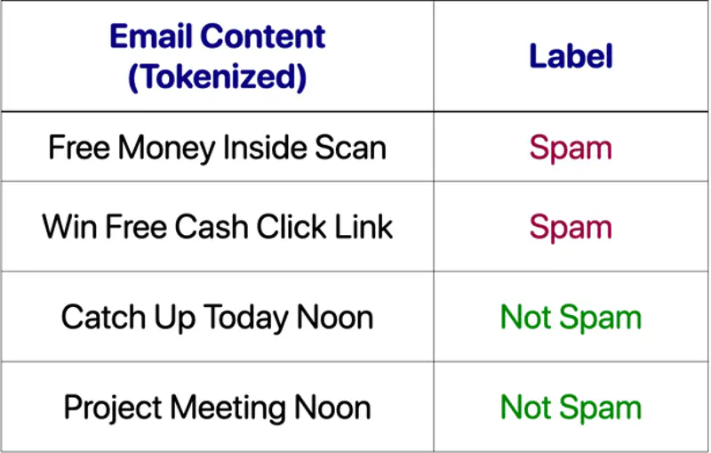
🏛️ Class Priors:
- P(Spam) = 2/4 =0.5
- P(Not Spam) = 2/4 = 0.5
📕 Vocabulary = { Free, Money, Inside, Scan, Win, Cash, Click, Link, Catch, Up Today, Noon, Project, Meeting }
- |V| = Total unique word count = 14
🧮 Class count:
- count(Spam) = 9
- count(Not Spam) = 7
✅ Laplace smoothing: \(\alpha = 1\)
- P(‘free’| Spam) = \(\frac{2+1}{9+14} = \frac{3}{23} = 0.13\)
- P(‘free’| Not Spam) = \(\frac{0+1}{7+14} = \frac{1}{21} = 0.047\)
👉 Say a new email 📧 arrives - “Free money today”; lets classify it as Spam/Not Spam.
Spam:
- P(‘free’| Spam) = \(\frac{2+1}{9+14} = \frac{3}{23} = 0.13\)
- P(‘money’| Spam) = \(\frac{1+1}{9+14} = \frac{2}{23} = 0.087\)
- P(‘today’| Spam) = \(\frac{0+1}{9+14} = \frac{1}{23} = 0.043\)
Not Spam:
- P(‘free’| Not Spam) = \(\frac{0+1}{7+14} = \frac{1}{21} = 0.047\)
- P(‘money’| Not Spam) = \(\frac{0+1}{7+14} = \frac{1}{21} = 0.047\)
- P(‘today’| Not Spam) = \(\frac{1+1}{7+14} = \frac{2}{21} = 0.095\)
- Score(Spam) = log(P(Spam)) + log(P(‘free’|S)) + log(P(‘money’|S)) + log(P(‘today’|S))
= log(0.5) + log(0.13) + log(0.087) + log(0.043) = -0.301 -0.886 -1.06 -1.366 = -3.614 - Score(Not Spam) = log(P(Not Spam)) + log(P(‘free’|NS)) + log(P(‘money’|NS)) + log(P(‘today’|NS))
= log(0.5) + log(0.047) + log(0.047) + log(0.095) = -0.301 -1.328 -1.328 -1.022 = -3.979
👉 Since, Score(Spam) (-3.614 )> Score(Not Spam) (-3.979) , the model chooses ‘Spam’ as the label for the email.
End of Section