This is the multi-page printable view of this section. Click here to print.
Decision Tree
1 - Decision Trees Introduction
💡It can be written as nested 🕸️ if else statements.
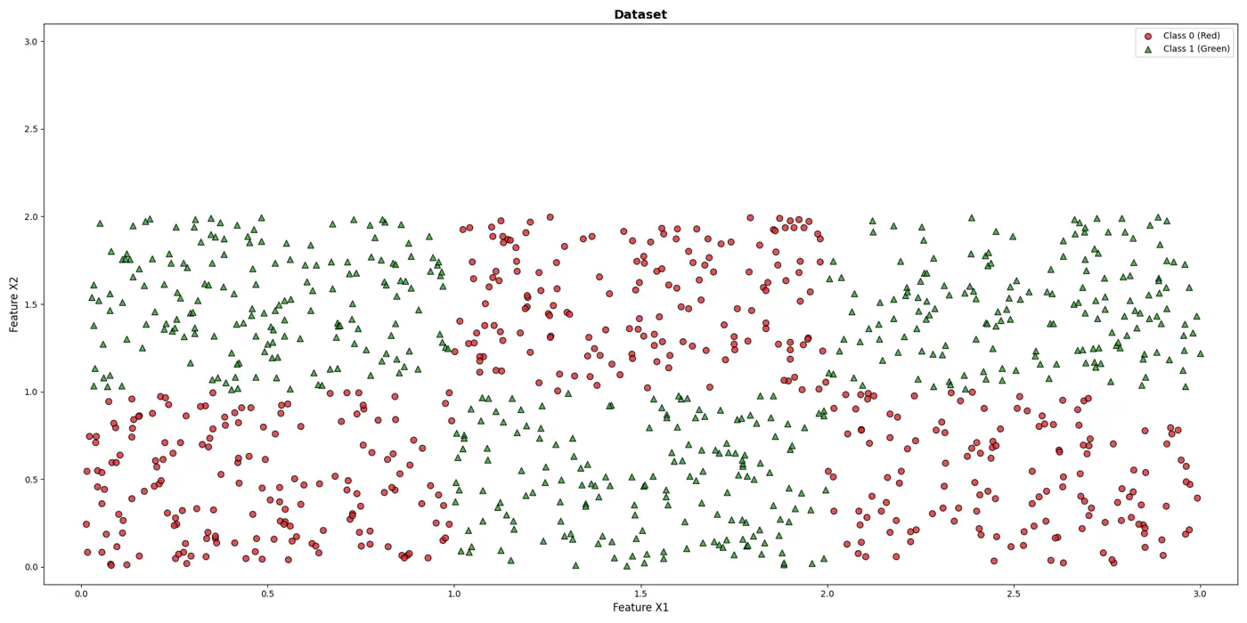
e.g: To classify the left bottom corner red points we can write:
👉if (FeatureX1 <1 & FeatureX2 <1)
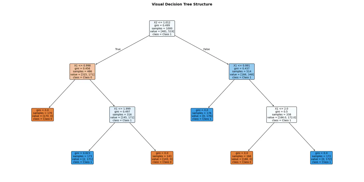
⭐️Extending the logic for all, we have an if else ladder like below:

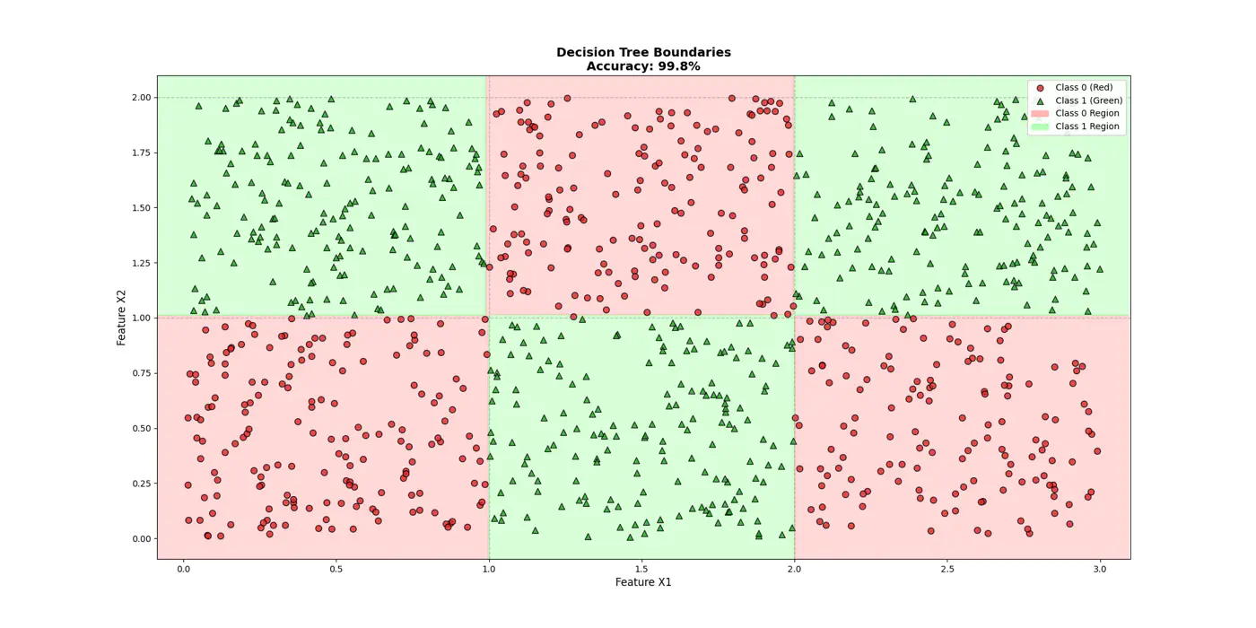
👉Final decision boundaries will be something like below:
- Non-parametric model.
- Recursively partitions the feature space.
- Top-down, greedy approach to iteratively select feature splits.
- Maximize purity of a node, based on metrics, such as, Information Gain 💵 or Gini 🧞♂️Impurity.
Note: We can extract the if/else logic of the decision tree and write in C++/Java for better performance.
⭐️Building an optimal decision tree 🌲 is a NP-Hard problem.
👉(Time Complexity: Exponential; combinatorial search space)
- Pros
- No standardization of data needed.
- Highly interpretable.
- Good runtime performance.
- Works for both classification & regression.
- Cons
- Number of dimensions should not be too large. (Curse of dimensionality)
- Overfitting.
- As base learners in ensembles, such as, bagging(RF), boosting(GBDT), stacking, cascading, etc.
- As a baseline, interpretable, model or for quick feature selection.
- Runtime performance is important.
End of Section
2 - Purity Metrics
Decision trees recursively partition the data based on feature values.
Pure Leaf 🍃 Node: Terminal node where every single data point belongs to the same class.
💡Zero Uncertainty.
The goal of a decision tree algorithm is to find the split that maximizes information gain, meaning it removes the most uncertainty from the data.
So, what is information gain ?
How do we reduce uncertainty ?
Let’s understand few terms first, before we understand information gain.
Measure ⏱ of uncertainty, randomness, or impurity in a data.
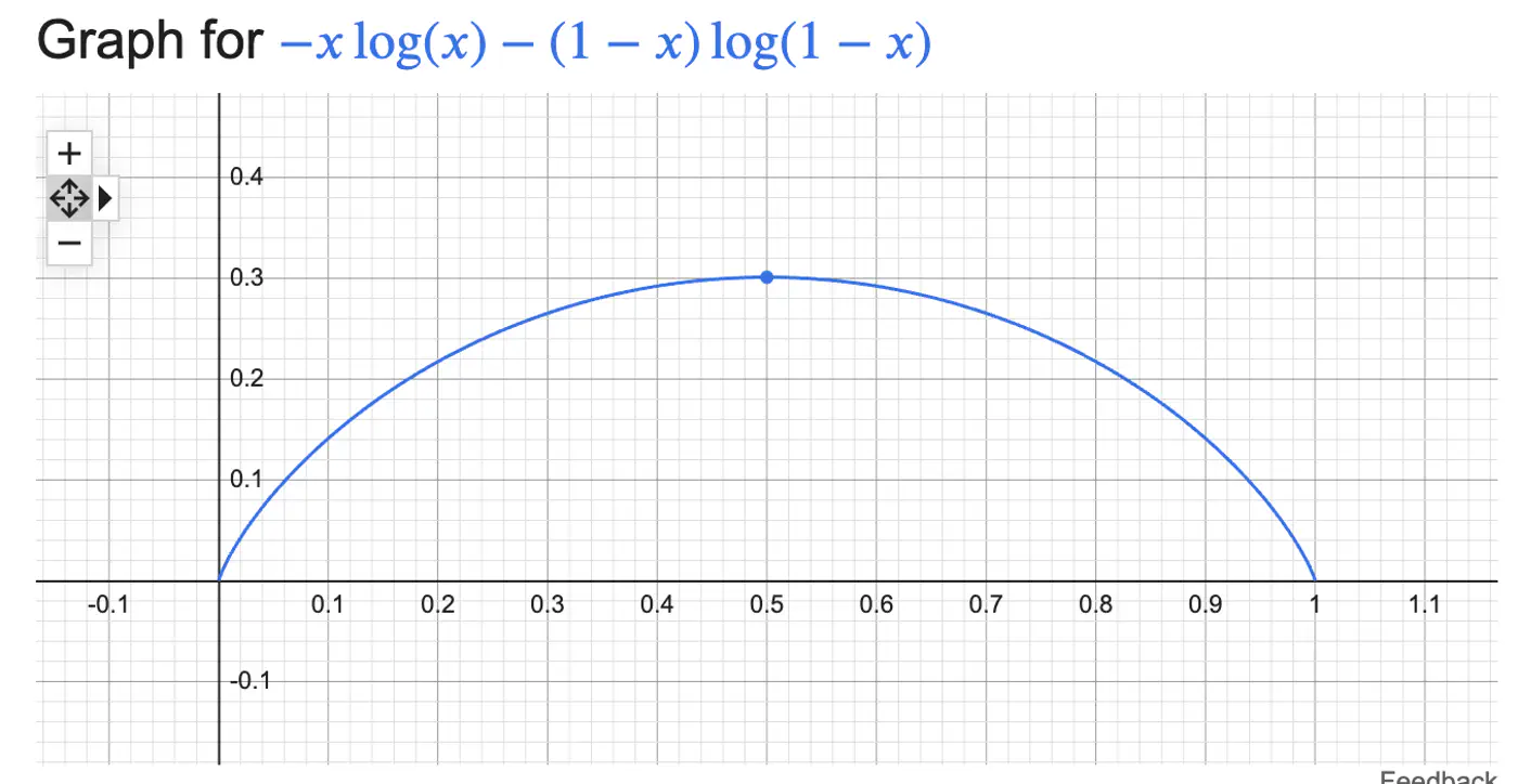
\[H(S)=-\sum _{i=1}^{n}p_{i}\log(p_{i})\]Binary Entropy:
💡Entropy can also be viewed as the ‘average surprise'.
A highly certain event provides little information when it occurs (low surprise).
An unlikely event provides a lot of information (high surprise).

⭐️ Measures the reduction in entropy (uncertainty) achieved by splitting a dataset based on a specific attribute.
\[IG=Entropy(Parent)-\left[\frac{N_{left}}{N_{parent}}Entropy(Child_{left})+\frac{N_{right}}{N_{parent}}Entropy(Child_{right})\right] \]Note: The goal of a decision tree algorithm is to find the split that maximizes information gain, meaning it removes the most uncertainty from the data.
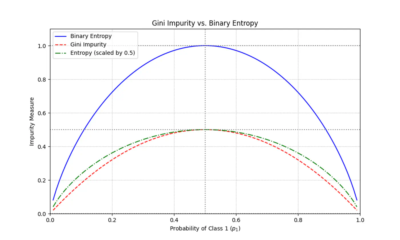
⭐️ Measures the probability of an element being incorrectly classified if it were randomly labeled according to the distribution of labels in a node.
\[Gini(S)=1-\sum_{i=1}^{n}(p_{i})^{2}\]- Range: 0 (Pure) - 0.5 (Maximum impurity)
Note: Gini is used in libraries like Scikit-Learn (as the default), because it avoids the computationally expensive 💰 log function.
Gini Impurity is a first-order approximation of Entropy.
For most of the real-world cases, choosing one over the other results in the exact same tree structure or negligible differences in accuracy.
When we plot the two functions, they follow nearly identical shapes.
End of Section
3 - Decision Trees For Regression
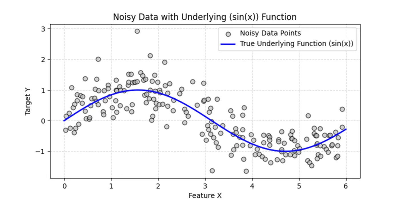
Decision Trees can also be used for Regression tasks but using a different metrics.
⭐️Metric:
- Mean Squared Error (MSE)
- Mean Absolute Error (MAE)
👉Say we have a following dataset, that we need to fit using decision trees:
👉Decision trees try to find the decision splits, building step functions that approximate the actual curve, as shown below:
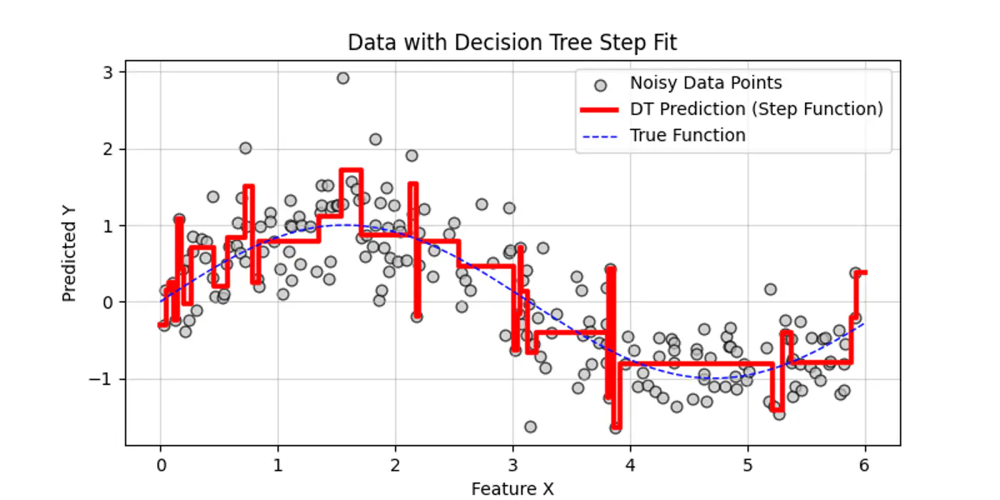
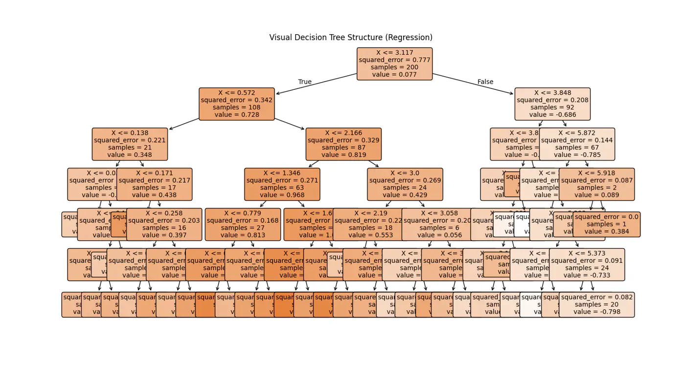
👉Internally the decision tree (if else ladder) looks like below:
Decision trees cannot predict values outside the range of the training data, i.e, extrapolation.
Let’s understand the interpolation and extrapolation cases one by one.
⭐️Predicting values within the range of features and targets observed during training 🏃♂️.
- Trees capture discontinuities perfectly, because they are piece-wise constant.
- They do not try to force a smooth line where a ‘jump’ exists in reality.
e.g: Predicting a house 🏡 price 💰 for a 3-BHK home when you have seen 2-BHK and 4-BHK homes in that same neighborhood.
⭐️Predicting values outside the range of training 🏃♂️data.
Problem:
Because a tree outputs the mean of training 🏃♂️ samples in a leaf, it cannot predict a value higher than the
highest ‘y’ it saw during training 🏃♂️.
- Flat-Line: Once a feature ‘X’ goes beyond the training boundaries, the tree falls into the same ‘last’ leaf forever.
e.g: Predicting the price 💰 of a house 🏡 in 2026 based on data from 2010 to 2025.
End of Section
4 - Regularization
- Pre-Pruning ✂️ &
- Post-Pruning ✂️
⭐️ ‘Early stopping’ heuristics (hyper-parameters).
- max_depth: Limits how many levels of ‘if else’ the tree can have; most common.
- min_samples_split: A node will only split, if it has at least ‘N’ samples; smooths the model (especially in regression), by ensuring predictions are based on an average of multiple points.
- max_leaf_nodes: Limiting the number of leaves reduces the overall complexity of the tree, making it simpler and less likely to memorize the training data’s noise.
- min_impurity_decrease: A split is only made if it reduces the impurity (Gini/MSE) by at least a certain threshold.
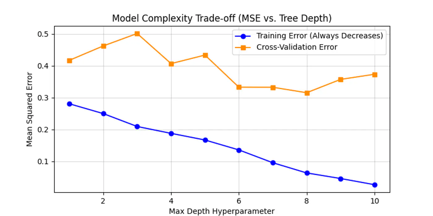
Below is an example for one of the hyper-parameter’s max_depth tuning.
As we can see below the cross-validation error decreases till depth=6 and after that reduction in error is not so significant.
Let the tree🌲 grow to its full depth (overfit) and then ‘collapse’ nodes that provide little predictive value.
Most common algorithm:
- Minimal Cost Complexity Pruning
💡Define a cost-complexity 💰 measure that penalizes the tree 🌲 for having too many leaves 🍃.
\[R_\alpha(T) = R(T) + \alpha |T|\]- R(T): total misclassification rate (or MSE) of the tree
- |T|: number of terminal nodes (leaves)
- \(\alpha\): complexity parameter (the ‘tax’ 💰 on complexity)
Logic:
- If \(\alpha\)=0, the tree is the original overfit tree.
- As \(\alpha\) increases 📈, the penalty for having many leaves grows 📈.
- To minimize the total cost 💰, the model is forced to prune branches that do not significantly reduce R(T).
- Use cross-validation to find the ‘sweet spot’ \(\alpha\) that minimizes validation error.
End of Section
5 - Bagging
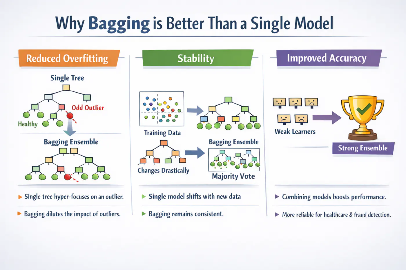
A single decision tree is highly sensitive to the specific training dataset.
Small changes, such as, a few different rows or the presence of an outlier, can lead to a completely different tree structure.Unpruned decision trees often grow until they perfectly classify the training set, essentially ‘memorizing’ noise and outliers, i.e, high variance, rather than finding general patterns.
Bagging = ‘Bootstrapped Aggregation’
Bagging 🎒is a parallel ensemble technique that reduces variance (without significantly increasing the bias) by training multiple versions of the same model on different random subsets of data and then combining their results.
Note: Bagging uses deep trees (overfit) and combines them to reduce variance.
Bootstrapping = ‘Without external help’
Given a training 🏃♂️set D of size ’n’, we create B new training sets D by sampling ’n’ observations from D ‘with replacement'.
💡Since, we are sampling ‘with replacement’, so, some data points may be picked multiple times, while others may not be picked at all.
- The probability that a specific observation is not selected in a bootstrap sample of size ’n’ is: \[\lim_{n \to \infty} \left(1 - \frac{1}{n}\right)^n = \frac{1}{e} \approx 0.368\]
🧐This means each tree is trained on roughly 63.2% of the unique data, while the remaining 36.8% (the Out-of-Bag or OOB set) can be used for cross validation.
⭐️Say we train ‘B’ models (base-learners), each with variance \(\sigma^2\) .
👉Average variance of ‘B’ models (trees) if all are independent:
\[Var(X)=\frac{\sigma^{2}}{B}\]👉Since, bootstrap samples are derived from the same dataset, the trees are correlated with some correlation coefficient ‘\(\rho\)'.
So, the true variance of bagged ensemble is:
\[Var(f_{bag}) = \rho \sigma^2 + \frac{1-\rho}{B} \sigma^2\]- \(\rho\)= 0; independent models, most reduction in variance.
- \(\rho\)= 1; fully correlated models, no improvement in variance.
- 0<\(\rho\)<1; As correlation decreases, variance reduces .
End of Section
6 - Random Forest
💡If one feature is extremely predictive (e.g., ‘Area’ for house prices), almost every bootstrap tree will split on that feature at the root.
👉This makes the trees(models) very similar, leading to a high correlation ‘\(\rho\)’.
\[Var(f_{bagging})=ρ\sigma^{2}+\frac{1-ρ}{B}\sigma^{2}\]💡Choose a random subset of ‘m’ features from the total ‘d’ features, reducing the correlation ‘\(\rho\)’ between trees.
👉By forcing trees to split on ‘sub-optimal’ features, we intentionally increase the variance of individual trees; also the bias is slightly increased (simpler trees).
Standard heuristics:
- Classification: \(m = \sqrt{d}\)
- Regression: \(m = \frac{d}{3}\)
💡Because ‘\(\rho\)’ is the dominant factor in the variance of the ensemble when B is large, the overall ensemble variance Var(\(f_{rf}\)) drops significantly lower than standard Bagging.
\[Var(f_{rf})=ρ\sigma^{2}+\frac{1-ρ}{B}\sigma^{2}\]💡A Random Forest will never overfit by adding more trees (B).
It only converges to the limit: ‘\(\rho\sigma^2\)’.
Overfitting is controlled by:
- depth of the individual trees.
- size of the feature subset ‘m'.
- High Dimensionality: 100s or 1000s of features; RF’s feature sampling prevents a few features from masking others.
- Tabular Data (with Complex Interactions): Captures non-linear relationships without needing manual feature engineering.
- Noisy Datasets: The averaging process makes RF robust to outliers (especially if using min_samples_leaf).
- Automatic Validation: Need a quick estimate of generalization error without doing 10-fold CV (via OOB Error).
End of Section
7 - Extra Trees
💡In a standard Decision Tree or Random Forest, the algorithm searches for the optimal split point (the threshold ’s’) that maximizes Information Gain or minimizes MSE.
👉This search is:
- computationally expensive (sort + mid-point) and
- tends to follow the noise in the training 🏃♂️data.
Adding randomness (right kind) in ensemble averaging reduces correlation/variance.
\[Var(f_{bag})=ρ\sigma^{2}+\frac{1-ρ}{B}\sigma^{2}\]- Random Thresholds: Instead of searching for the best split point (computationally expensive 💰) for a feature, it picks a threshold at random from a uniform distribution between the feature’s local minimum and maximum.
- Entire Dataset: Uses entire training dataset (default) for every tree; no bootstrapping.
- Random Feature Subsets: Random subset of m<n features is used in each decision tree.
Picking thresholds randomly has two effects:
- Structural correlation between trees becomes extremely low.
- Individual trees are ‘weaker’ and have higher bias than a standard optimized tree.
👉The massive drop in ‘\(\rho\)’ often outweighs the slight increase in bias, leading to an overall ensemble that is smoother and more robust to noise than a standard Random Forest.
Note: Extra Trees are almost always grown to full depth, as they may need extra splits to find the same decision boundary.
- Performance: Significantly faster to train, as it does not sort data to find optimal split.
Note: If we are working with billions of rows or thousands of features, ET can be 3x to 5x faster than a Random Forest(RF). - Robustness to Noise: By picking thresholds randomly, tends to ‘handle’ the noise more effectively than RF.
- Feature Importance: Because ET is so randomized, it often provides more ‘stable’ feature importance scores.
Note: It is less likely to favor a high-cardinality feature (e.g. zip-code) just because it has more potential split points.
End of Section
8 - Boosting
⭐️In Bagging 🎒we trained multiple strong(over-fit, high variance) models (in parallel) and then averaged them out to reduce variance.
💡Similarly, we can train many weak(under-fit, high bias) models sequentially, such that, each new model corrects the errors of the previous ones to reduce bias.
⚔️ An ensemble learning approach where multiple ‘weak learners’ (typically simple models like shallow decision trees 🌲 or ‘stumps’) are sequentially combined to create a single strong predictive model.
⭐️The core principle is that each subsequent model focuses 🎧 on correcting the errors made by its predecessors.
- AdaBoost(Adaptive Boosting)
- Gradient Boosting Machine (GBM)
- XGBoost
- LightGBM (Microsoft)
- CatBoost (Yandex)
End of Section
9 - AdaBoost
💡Works by increasing 📈 the weight 🏋️♀️ of misclassified data points after each iteration, forcing the next weak learner to ‘pay more attention’🚨 to the difficult cases.
⭐️ Commonly used for classification.
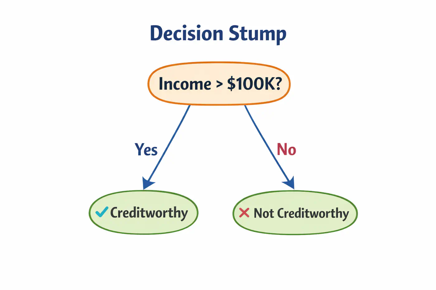
👉Weak learners are typically ‘Decision Stumps’, i.e, decision trees🌲with a depth of only one (1 split, 2 leaves 🍃).
- Assign an equal weight 🏋️♀️to every data point; \(w_i = 1/n\), where ’n’=number of samples.
- Build a decision stump that minimizes the weighted classification error.
- Calculate total error; \(E_m = \Sigma w_i\).
- Determine ‘amount of say’, i.e, the weight 🏋️♀️ of each stump in final decision.
\[\alpha_m = \frac{1}{2}ln\left( \frac{1-E_m}{E_m} \right)\]
- Low error results in a high positive \(\alpha\) (high influence).
- 50% error (random guessing) results in an \(\alpha = 0\) (no influence).
- Update sample weights 🏋️♀️.
- Misclassified samples: Weight 🏋️♀️ increases by \(e^{\alpha_m}\).
- Correctly classified samples: Weight 🏋️♀️ decreases by \(e^{-\alpha_m}\).
- Normalization: All new weights 🏋️♀️ are divided by their total sum so they add up back to 1.
- Iterate for a specified number of estimators (n_estimators).
👉 To classify a new data point, every stump makes a prediction (+1 or -1).
These are multiplied by their respective ‘amount of say’ \(\alpha_m\) and summed.
\[H(x)=sign\sum_{m=1}^{M}\alpha_{m}⋅h_{m}(x)\]👉 If the total weighted 🏋️♀️ sum is positive, the final class is +1; otherwise -1.
Note: Sensitive to outliers; Because AdaBoost aggressively increases weights 🏋️♀️ on misclassified points, it may ‘over-focus’ on noisy outliers, hurting performance.
End of Section
10 - Gradient Boosting Machine
GBM treats the final model \(F_m(x)\) as weighted 🏋️♀️ sum of ‘m’ weak learners:
\[ F_{M}(x)=\underbrace{F_{0}(x)}_{\text{Initial\ Guess}}+\nu \sum _{m=1}^{M}\underbrace{\left(\sum _{j=1}^{J_{m}}\gamma _{jm}\mathbb{I}(x\in R_{jm})\right)}_{\text{Weak\ Learner\ }h_{m}(x)}\]- \(F_0(x)\): The initial base model (usually a constant).
- M: The total number of boosting iterations (number of trees).
- \(\gamma_{jm}\)(Leaf Weight): The optimized value for leaf in tree .
- \(\nu\)(Nu): The Learning Rate or Shrinkage; prevent overfitting.
- \(\mathbb{I}(x\in R_{jm})\): ‘Indicator Function’; It is 1 if data point falls into leaf of the tree, and 0 otherwise.
- \(R_{jm}\)(Regions): Region of \(j_{th}\) leaf in \(m_{th}\)tree.
📍In Gradient Descent, we update parameters ‘\(\Theta\)';
📍In GBM, we update the predictions F(x) themselves.
🦕We move the predictions in the direction of the negative gradient of the loss function L(y, F(x)).
🎯We want to minimize loss:
\[\mathcal{L}(F) = \sum_{i=1}^n L(y_i, F(x_i))\]✅ In parameter optimization we update weights 🏋️♀️:
\[w_{t+1} = w_t - \eta \cdot \nabla_{w}\mathcal{L}(w_t)\]✅ In gradient boosting, we update the prediction function:
\[F_m(x) = F_{m-1}(x) -\eta \cdot \nabla_F \mathcal{L}(F_{m-1}(x))\]➡️ The gradient is calculated w.r.t. predictions, not weights.
In GBM we can use any loss function as long as it is differentiable, such as, MSE, log loss, etc.
Loss(MSE) = \((y_i - F_m(x_i))^2\)
\[\frac{\partial L}{F_m(x_i)} = -2 (y-F_m(x_i))\]\[\implies \frac{\partial L}{F_m(x_i)} \propto - (y-F_m(x_i))\]👉Pseudo Residual (Error) = - Gradient
💡To minimize loss, take derivative of loss function w.r.t ‘\(\gamma\)’ and equate to 0:
\[F_0(x) = \arg\min_{\gamma} \sum_{i=1}^n L(y_i, \gamma)\]MSE Loss = \(\mathcal{L}(y_i, \gamma) = \sum_{i=1}^n(y_i -\gamma)^2\)
\[ \begin{aligned} &\frac{\partial \mathcal{L}(y_i, \gamma)}{\partial \gamma} = -2 \cdot \sum_{i=1}^n(y_i -\gamma) = 0 \\ &\implies \sum_{i=1}^n (y_i -\gamma) = 0 \\ &\implies \sum_{i=1}^n y_i = n.\gamma \\ &\therefore \gamma = \frac{1}{n} \sum_{i=1}^n y_i \end{aligned} \]💡To minimize cost, take derivative of cost function w.r.t ‘\(\gamma\)’ and equate to 0:
Cost Function = \(J(\gamma )\)
\[J(\gamma )=\sum _{x_{i}\in R_{jm}}\frac{1}{2}(y_{i}-(F_{m-1}(x_{i})+\gamma ))^{2}\]We know that:
\[ r_{i}=y_{i}-F_{m-1}(x_{i})\]\[\implies J(\gamma )=\sum _{x_{i}\in R_{jm}}\frac{1}{2}(r_{i}-\gamma )^{2}\]\[\frac{d}{d\gamma }\sum _{x_{i}\in R_{jm}}\frac{1}{2}(r_{i}-\gamma )^{2}=\sum _{x_{i}\in R_{jm}}-(r_{i}-\gamma )=0\]\[\implies \sum _{x_{i}\in R_{jm}}\gamma -\sum _{x_{i}\in R_{jm}}r_{i}=0\]👉Since, \(\gamma\) is constant for all \(n_j\) samples in the leaf, \(\sum _{x_{i}\in R_{jm}}\gamma =n_{j}\gamma \)
\[n_{j}\gamma =\sum _{x_{i}\in R_{jm}}r_{i}\]\[\implies \gamma =\frac{\sum _{x_{i}\in R_{jm}}r_{i}}{n_{j}}\]Therefore, \(\gamma\) = average of all residuals in the leaf.
Note: \(R_{jm}\)(Regions): Region of \(j_{th}\) leaf in \(m_{th}\)tree.
End of Section
11 - GBDT Algorithm
Gradient Boosted Decision Tree (GBDT) is a decision tree based implementation of Gradient Boosting Machine (GBM).
GBM treats the final model \(F_m(x)\) as weighted 🏋️♀️ sum of ‘m’ weak learners (decision trees):
\[ F_{M}(x)=\underbrace{F_{0}(x)}_{\text{Initial\ Guess}}+\nu \sum _{m=1}^{M}\underbrace{\left(\sum _{j=1}^{J_{m}}\gamma _{jm}\mathbb{I}(x\in R_{jm})\right)}_{\text{Decision\ Tree\ }h_{m}(x)}\]- \(F_0(x)\): The initial base model (usually a constant).
- M: The total number of boosting iterations (number of trees).
- \(\gamma_{jm}\)(Leaf Weight): The optimized value for leaf in tree .
- \(\nu\)(Nu): The Learning Rate or Shrinkage; prevent overfitting.
- \(\mathbb{I}(x\in R_{jm})\): ‘Indicator Function’; It is 1 if data point falls into leaf of the tree, and 0 otherwise.
- \(R_{jm}\)(Regions): Region of \(j_{th}\) leaf in \(m_{th}\)tree.
- Step 1: Initialization.
- Step 2: Iterative loop 🔁 : for i=1 to m.
- 2.1: Calculate pseudo residuals ‘\(r_{im}\)'.
- 2.2: Fit a regression tree 🌲‘\(h_m(x)\)'.
- 2.3:Compute leaf 🍃weights 🏋️♀️ ‘\(\gamma_{jm}\)'.
- 2.4:Update the model.
Start with a function that minimizes our loss function;
for MSE its mean.
MSE Loss = \(\mathcal{L}(y_i, \gamma) = \sum_{i=1}^n(y_i -\gamma)^2\)
Find the ‘gradient’ of error;
Tells us the direction and magnitude needed to reduce the loss.
Train a tree to predict the residuals ‘\(h_m(x)\)';
- Tree 🌲 partitions the data into leaves 🍃 (\(R_{jm}\)regions )
Within each leaf 🍃, we calculate the optimal value ‘\(\gamma_{jm}\)’ that minimizes the loss for the samples in that leaf 🍃.
\[\gamma_{jm} = \arg\min_{\gamma} \sum_{x_i \in R_{jm}} L(y_i, F_{m-1}(x_i) + \gamma)\]➡️ The optimal leaf 🍃value is the ‘Mean’(MSE) of the residuals; \(\gamma = \frac{\sum r_i}{n_j}\)
Add the new ‘correction’ to the existing model, scaled by the learning rate.
\[F_{m}(x)=F_{m-1}(x)+\nu \cdot \underbrace{\sum _{j=1}^{J_{m}}\gamma _{jm}\mathbb{I}(x\in R_{jm})}_{h_{m}(x)}\]- \(\mathbb{I}(x\in R_{jm})\): ‘Indicator Function’; It is 1 if data point falls into leaf of the tree, and 0 otherwise.
End of Section
12 - GBDT Example
Gradient Boosted Decision Tree (GBDT) is a decision tree based implementation of Gradient Boosting Machine (GBM).
GBM treats the final model \(F_m(x)\) as weighted 🏋️♀️ sum of ‘m’ weak learners (decision trees):
\[ F_{M}(x)=\underbrace{F_{0}(x)}_{\text{Initial\ Guess}}+\nu \sum _{m=1}^{M}\underbrace{\left(\sum _{j=1}^{J_{m}}\gamma _{jm}\mathbb{I}(x\in R_{jm})\right)}_{\text{Decision\ Tree\ }h_{m}(x)}\]- \(F_0(x)\): The initial base model (usually a constant).
- M: The total number of boosting iterations (number of trees).
- \(\gamma_{jm}\)(Leaf Weight): The optimized value for leaf in tree .
- \(\nu\)(Nu): The Learning Rate or Shrinkage; prevent overfitting.
- \(\mathbb{I}(x\in R_{jm})\): ‘Indicator Function’; It is 1 if data point falls into leaf of the tree, and 0 otherwise.
- \(R_{jm}\)(Regions): Region of \(j_{th}\) leaf in \(m_{th}\)tree.
- Step 1: Initialization.
- Step 2: Iterative loop 🔁 : for i=1 to m.
- 2.1: Calculate pseudo residuals ‘\(r_{im}\)'.
- 2.2: Fit a regression tree 🌲‘\(h_m(x)\)'.
- 2.3:Compute leaf 🍃weights 🏋️♀️ ‘\(\gamma_{jm}\)'.
- 2.4:Update the model.
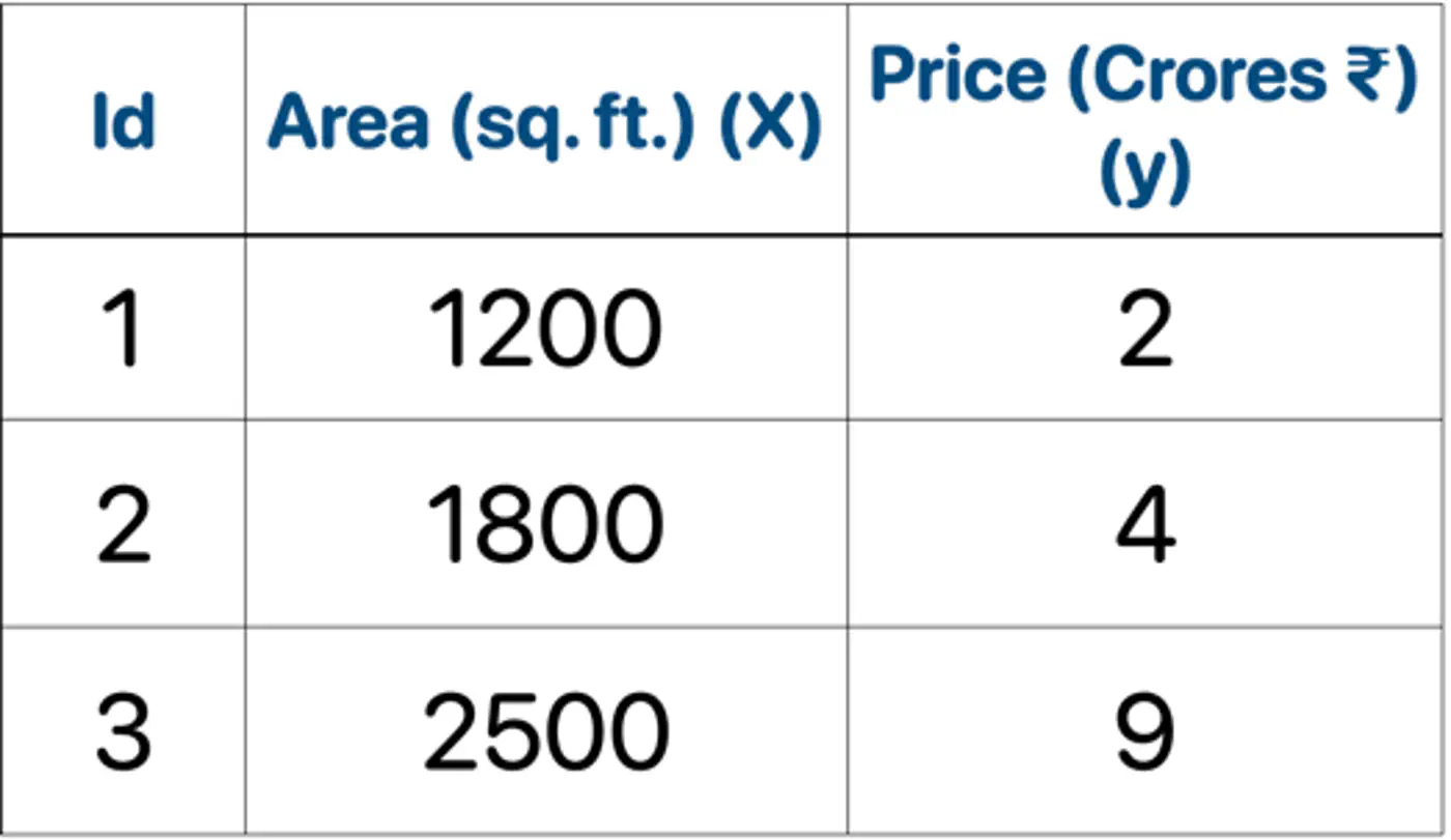
👉Loss = MSE, Learning rate (\(\nu\)) = 0.5
- Initialization : \(F_0(x) = mean(2,4,9) = 5.0\)
- Iteration 1(m=1):
2.1: Calculate residuals ‘\(r_{i1}\)'
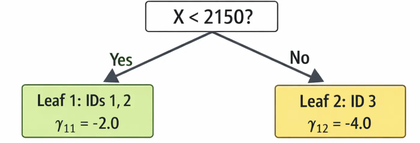
\[\begin{aligned} r_{11} &= 2-5 = -3.0 \\ r_{21} &= 4-5 = -1.0 \\ r_{31} &= 9-5 = 4.0 \\ \end{aligned} \]2.2: Fit tree(\(h_1\)); Split at X<2150 (midpoint of 1800 and 2500)
2.3: Compute leaf weights \(\gamma_{j1}\)
- Y-> Leaf 1: Ids 1, 2 ( \(\gamma_{11}\)= -2.0)
- N-> Leaf 2: Id 3 ( \(\gamma_{21}\)= 4.0)
2.4: Update predictions (\(F_1 = F_0 + 0.5 \cdot \gamma\))
\[ \begin{aligned} F_1(x_1) &= 5.0 + 0.5(-2.0) = \mathbf{4.0}\ \\F_1(x_2) &= 5.0 + 0.5(-2.0) = \mathbf{4.0}\ \\F_1(x_3) &= 5.0 + 0.5(4.0) = \mathbf{7.0}\ \\ \end{aligned} \]Tree 1:
- Iteration 2(m=2):
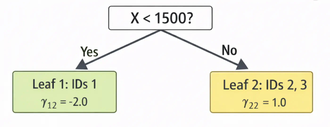
2.1: Calculate residuals ‘\(r_{i2}\)'
\[ \begin{aligned} r_{12} &= 2-4.0 = -2.0 \\ r_{22} &= 4-4.0 = 0.0 \\ r_{32} &= 9-7.0 = 2.0 \\ \end{aligned} \]2.2: Fit tree(\(h_2\)); Split at X<1500 (midpoint of 1200 and 1800)
2.3: Compute leaf weights \(\gamma_{j2}\)
- Y-> Leaf 1: Ids 1 ( \(\gamma_{12}\)= -2.0)
- N-> Leaf 2: Id 2, 3 ( \(\gamma_{22}\)= 1.0)
2.4: Update predictions (\(F_1 = F_0 + 0.5 \cdot \gamma\))
\[ \begin{aligned} F_2(x_1) &= 4.0 + 0.5(-2.0) = \mathbf{3.0} \\F_2(x_2) &= 4.0 + 0.5(1.0) = \mathbf{4.5} \\ F_2(x_3) &= 7.0 + 0.5(1.0) = \mathbf{7.5}\ \\ \end{aligned} \]Tree 2:
Note: We can keep adding more trees with every iteration;
ideally, learning rate \(\nu\) is small, say 0.1, so that we do not overshoot and converge slowly.
Let’s predict the price of a house with area = 2000 sq. ft.
- \(F_{0}=5.0\)
- Pass though tree 1 (\(h_1\)): is 2000 < 2150 ? Yes, \(\gamma_{11}\)= -2.0
- Contribution (\(h_1\)) = 0.5 x (-2.0) = -1.0
- Pass though tree 2 (\(h_2\)): is 2000 < 1500 ? No, \(\gamma_{22}\) = 1.0
- Contribution(\(h_2\)) = 0.5 x (1.0) = 0.5
- Final prediction = 5.0 - 1.0 + 0.5 = 4.5
Therefore, the price of a house with area = 2000 sq. ft is Rs 4.5 crores, which is very close.
In just 2 iterations, although with higher learning rate (\(\nu=0.5\)), we were able to get a fairly good estimate.
End of Section
13 - Advanced GBDT Algorithms
🔵 LightGBM (Light Gradient Boosting Machine)
⚫️ CatBoost (Categorical Boosting)
⭐️An optimized and highly efficient implementation of gradient boosting.
👉 Widely used in competitive data science (like Kaggle) due to its speed and performance.
Note: Research project developed by Tianqi Chen during his doctoral studies at the University of Washington.
⭐️Developed by Microsoft, this framework is designed for high speed and efficiency with large datasets.
👉It grows trees leaf-wise rather than level-wise and uses Gradient-based One-Side Sampling (GOSS) to speed 🐇 up the finding of optimal split points.
End of Section
14 - XgBoost
⭐️An optimized and highly efficient implementation of gradient boosting.
👉 Widely used in competitive data science (like Kaggle) due to its speed and performance.
Note: Research project developed by Tianqi Chen during his doctoral studies at the University of Washington.
🔵 Regularization
🔵 Sparsity-Aware Split Finding
⭐️Uses second derivative (Hessian), i.e, curvature, in addition to first derivative (gradient) to optimize the objective function more quickly and accurately than GBDT.
Let’s understand this with the problem to minimize \(f(x) = x^4\), using:
Gradient descent (uses only 1st order derivative, \(f'(x) = 4x^3\))
Newton’s method (uses both 1st and 2nd order derivatives \(f''(x) = 12x^2\))

- Adds explicit regularization terms (L1/L2 on leaf weights and tree complexity) into the boosting objective, helping reduce over-fitting. \[ \text{Objective} = \underbrace{\sum_{i=1}^{n} L(y_i, \hat{y}_i)}_{\text{Training Loss}} + \underbrace{\gamma T + \frac{1}{2}\lambda \sum_{j=1}^{T} w_j^2 + \alpha \sum_{j=1}^{T} |w_j|}_{\text{Regularization (The Tax)}} \]
💡Real-world data often contains many missing values or zero-entries (sparse data).
👉 XGBoost introduces a ‘default direction’ for each node.
➡️During training, it learns the best direction (left or right) for missing values to go, making it significantly faster and more robust when dealing with sparse or missing data.
End of Section
15 - LightGBM
⭐️Developed by Microsoft, this framework is designed for high speed and efficiency with large datasets.
👉It grows trees leaf-wise rather than level-wise and uses Gradient-based One-Side Sampling (GOSS) to speed 🐇 up the finding of optimal split points.
🔵 Exclusive Feature Bundling (EFB)
🔵 Leaf-wise Tree Growth Strategy
- ❌ Traditional GBDT uses all data instances for gradient calculation, which is inefficient.
- ✅ GOSS focuses 🔬on instances with larger gradients (those that are less well-learned or have higher error).
- 🐛 Keeps all instances with large gradients but randomly samples from those with small gradients.
- 🦩This way, it prioritizes the most informative examples for training, significantly reducing the data used and speeding up 🐇 the process while maintaining accuracy.
- 🦀 High-dimensional data often contains many sparse, mutually exclusive features (features that never take a non-zero value simultaneously, such as, One Hot Encoding (OHE)).
- 💡 EFB bundles the non-overlapping features into a single, dense feature, reducing the number of features, without losing much information, saving computation.
- ❌ Traditional gradient boosting machines (like XGBoost), the trees are built level-wise (BFS-like), meaning all nodes at the current level are split before moving to the next level.
- ✅ LightGBM maintains a set of all potential leaves that can be split at any given time and selects the leaf (for splitting) that provides the maximum gain across the entire tree, regardless of its depth.
Note: Need mechanisms to avoid over-fitting.
End of Section
16 - CatBoost
🔵 Symmetric(Oblivious) Trees
🔵 Handling Missing Values
- ❌ Standard target encoding can lead to target leakage, where the model uses information from the target variable during training that would not be available during inference.
👉(model ‘cheats’ by using a row’s own label to predict itself). - ✅ CatBoost calculates the target statistics (average target value) for each category based only on the history of previous training examples in a random permutation of the data.
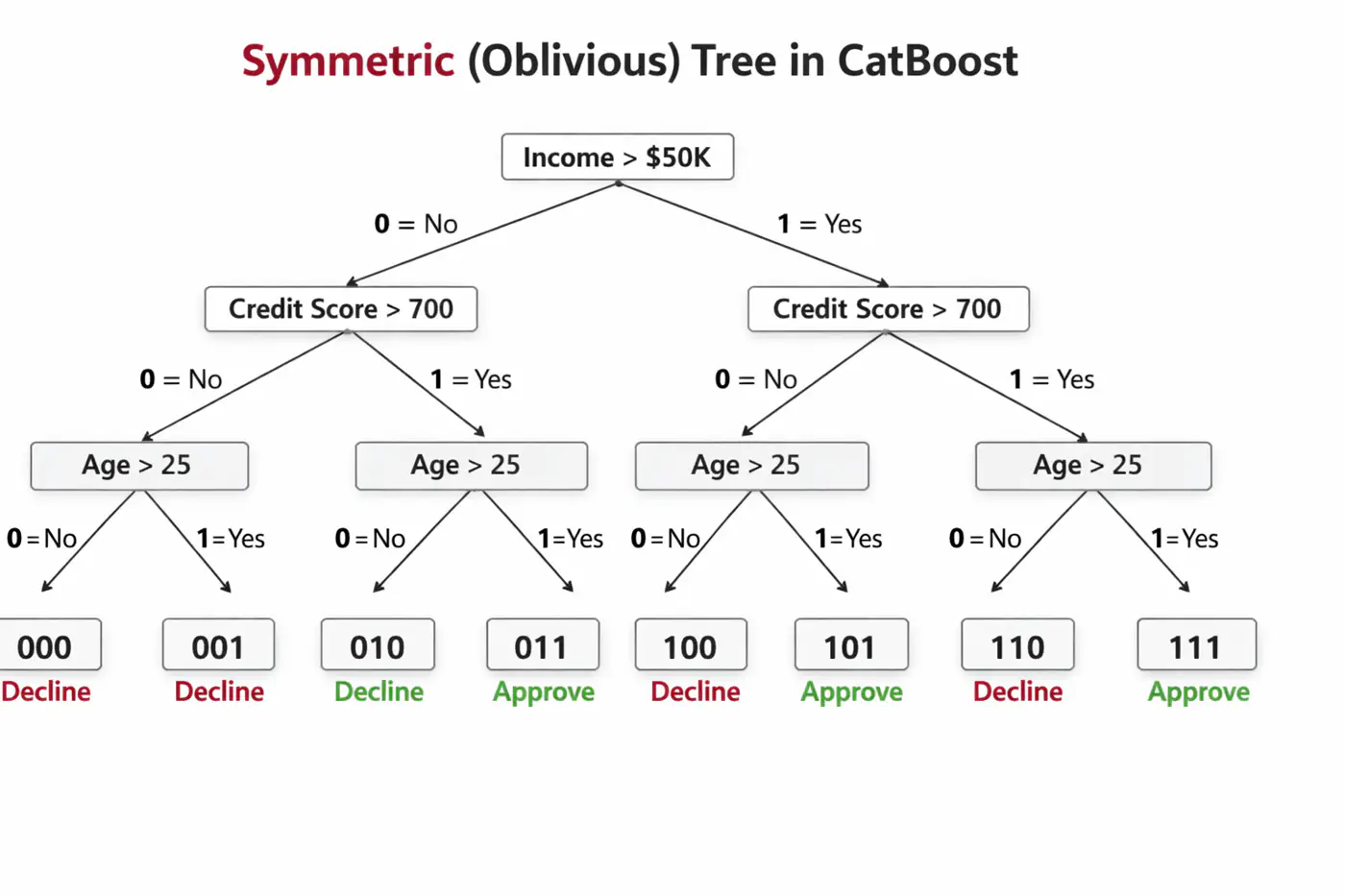
🦋 Uses symmetric decision trees by default.
👉 In symmetric trees, the same split condition is applied at each level across the entire tree structure.🦘Does not walk down the tree using ‘if-else’ logic, instead it evaluates decision conditions to create a binary index (e.g 101) and jumps directly to that leaf 🍃 in memory 🧠.
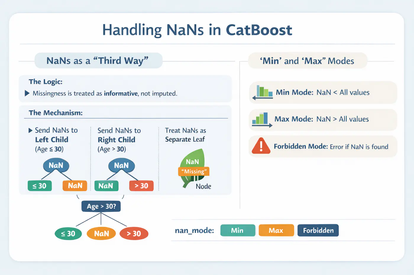
⚙️ CatBoost offers built-in, intelligent handling of missing values and sparse features, which often require manual preprocessing in other GBDT libraries.
💡Treats ‘NaN’ as a distinct category, reducing the need for imputation.
End of Section