• Parametric models:
  • Rely on assumption that relationships between data points are linear.
  • For polynomial regression we need to find the degree of polynomial.
• Training:
  • We need to train 🏃‍♂️the model for prediction.

• Simple: Intuitive way to classify data or predict values by finding similar existing data points (neighbors).

• Non-Parametric: Makes no assumptions about the underlying data distribution.

• No Training Required: KNN is a ‘lazy learner’, it does not require a formal training 🏃‍♂️ phase.

  

  

Given a query point \(x_q\) and a dataset, D = {\((x_i,y_i)_{i=1}^n, \quad x_i,y_i \in \mathbb{R}^d\)}, the algorithm finds a set of ‘k’ nearest neighbors \(\mathcal{N}_k(x_q) \subseteq D\).

Inference:

1. Choose a value of ‘k’ (hyper-parameter); odd number.
2. Calculate distance (Euclidean, Cosine etc.) between and every point in dataset and store in a distance list.
3. Sort the distance list in ascending order; choose top ‘k’ data points.
4. Make prediction:
   • Classification: Take majority vote of ‘k’ nearest neighbors and assign label.
   • Regression: Take the mean/median of ‘k’ nearest neighbors.

Note: Store entire dataset.

• Storing Data: Space Complexity: O(nd)
• Inference: Time Complexity ⏰: O(nd + nlogn)

Explanation:

• Distance to all ’n’ points in ‘d’ dimensions: O(nd)
• Sorting all ’n’ data points : O(nlogn)

Note: Brute force 🔨 KNN is unacceptable when ’n’ is very large, say billions.

Naive KNN needs some improvements to fix some of its drawbacks.

• Standardization
• Distance-Weighted KNN
• Mahalanobis Distance

⭐️Say one feature is ‘Annual Income’ (0-1M), and another feature is ‘Years of Experience’ (0-40).

👉The Euclidean distance will be almost entirely dominated by income 💵.

💡So, we do standardization of each feature, such that it has a mean, \(\mu\)=0 and variance,\(\sigma\)=1.

⭐️Vanilla KNN treats the 1st nearest neighbor and the k-th nearest neighbor as equal.

💡A neighbor that is 0.1units away should have more influence than a neighbor that is 10 units away.

👉We assign weight 🏋️‍♀️ to each neighbor; most common strategy is inverse of squared distance.

Improvements:

• Noise/Outlier: Reduces the impact of ‘noise’ or ‘outlier’ (distant neighbors).
• Imbalanced Data: Closer points dominate, mitigating impact of imbalanced data.
  • e.g: If you have a query point surrounded by 2 very close ‘Class A’ points and 3 distant ‘Class B’ points, weighted 🏋️‍♀️ KNN will correctly pick ‘Class A'.

⭐️Euclidean distance makes assumption that all the features are independent and provide unique information.

💡‘Height’ and ‘Weight’ are highly correlated.

👉If we use Euclidean distance, we are effectively ‘double-counting’ the size of the person.

🏇Mahalanobis distance measures distance in terms of standard deviations from the mean, accounting for the covariance between features.

\(\Sigma\): Covariance matrix of the data

• If \(\Sigma\) is identity matrix, Mahalanobis distance reduces to Euclidean distance.
• If \(\Sigma\) is a diagonal matrix, Mahalanobis distance reduces to Normalized Euclidean distance.

🦀Naive KNN shifts all computation 💻 to inference time ⏰, and it is very slow.

• To find the neighbor for one query, we must touch every single bit of the ‘nxd’ matrix.
• If n=10^9,a single query would take seconds, but we need milliseconds.

• Distance Weighted KNN
  • K-D Trees (d<20): Recursively partitions space into axis-aligned hyper-rectangles. O(log N ) search.
  • Ball Trees : High dimensional data; Haversine distance for geospatial 🌎 data.
• Approximate Nearest Neighbors (ANN)
  • Locality Sensitive Hashing (LSH): Uses ‘bucketizing’ 🗑️ hashes. Points that are close have a high probability of having the same hash.
  • Hierarchical Navigable Small World (HNSW); Graph of vectors; Search is a ‘greedy walk’ across levels.
• Product Quantization (Reduce memory 🧠 footprint 👣 of high dimensional vectors)
  • ScaNN (Google)
  • FAISS (Meta)
• Dimensionality Reduction (Mitigate ‘Curse of Dimensionality’)
  • PCA

While Euclidean distance(L norm) is the most frequently discussed, ‘Curse of Dimensionality’ impacts all Minkowski norms (\(L_p\))

Note: ‘Curse of Dimensionality’ is largely a function of the exponent (p) in the distance calculation.

Coined 🪙 by mathematician John Bellman in the 1960s while studying dynamic programming.

High dimensional data created following challenges:

• Distance Concentration
• Data Sparsity
• Exponential Sample Requirement

💡Consider a hypercube in d-dimensions of side length = 1; Volume = \(1^d\) = 1
🧊 A smaller inner cube with side length = 1 - \(\epsilon\) ; Volume = \((1 -\epsilon)^d\)

🧐 This implies that almost all the volume of the high-dimensional cube lies near the ‘crust’.
👉e.g: if \(\epsilon\)= 0.01, d = 500; Volume of inner cube = \((1 -0.01)^{500}\) = \(0.99^{500}\) = 0.006 = 0.6%
🤔Consequently, all points become nearly equidistant, and the concept of ‘nearest’ or ‘neighborhood’ loses its meaning.

⭐️The volume of the feature space increases exponentially with each added dimension.

👉To maintain the same data density found in a 1D space with 10 points, we would need \(10^{10}\)(10 billion) points in 10D space.

💡Because real-world datasets are rarely this large, the data becomes “sparse,” making it difficult to find truly similar neighbors.

⭐️To maintain a reliable result, the amount of training data needed must grow exponentially with the number of dimensions.

👉Without this growth, the model is highly prone to overfitting, where it learns from noise in the ‘sparse’ data rather than actual underlying patterns.

Note: For modern embeddings (often 768 or 1536 dimensions), it is mathematically impossible to collect enough data to ‘fill’ the space.

• Cosine Similarity
• Normalization

Cosine similarity measures the cosine of the angle between 2 vectors.

Note: Cosine similarity mitigates the ‘curse of dimensionality" problem.

⭐️Normalize the vector, i.e, make its length =1, a unit vector.

💡By normalizing, we project all points onto the surface of a unit hypersphere.

• We are no longer searching in the ‘empty’ high-dimensional volume of a hypercube.
• Now, we are searching on a constrained manifold (the shell).

Note: By normalizing, we move the data from the volume of the D-dimensional space onto the surface of a (D-1)-dimensional hypersphere.

Euclidean Distance Squared of Normalized Vectors:

Note: This formula proves that maximizing ‘Cosine similarity’ is identical to minimizing ‘Euclidean distance’ on the hypersphere.

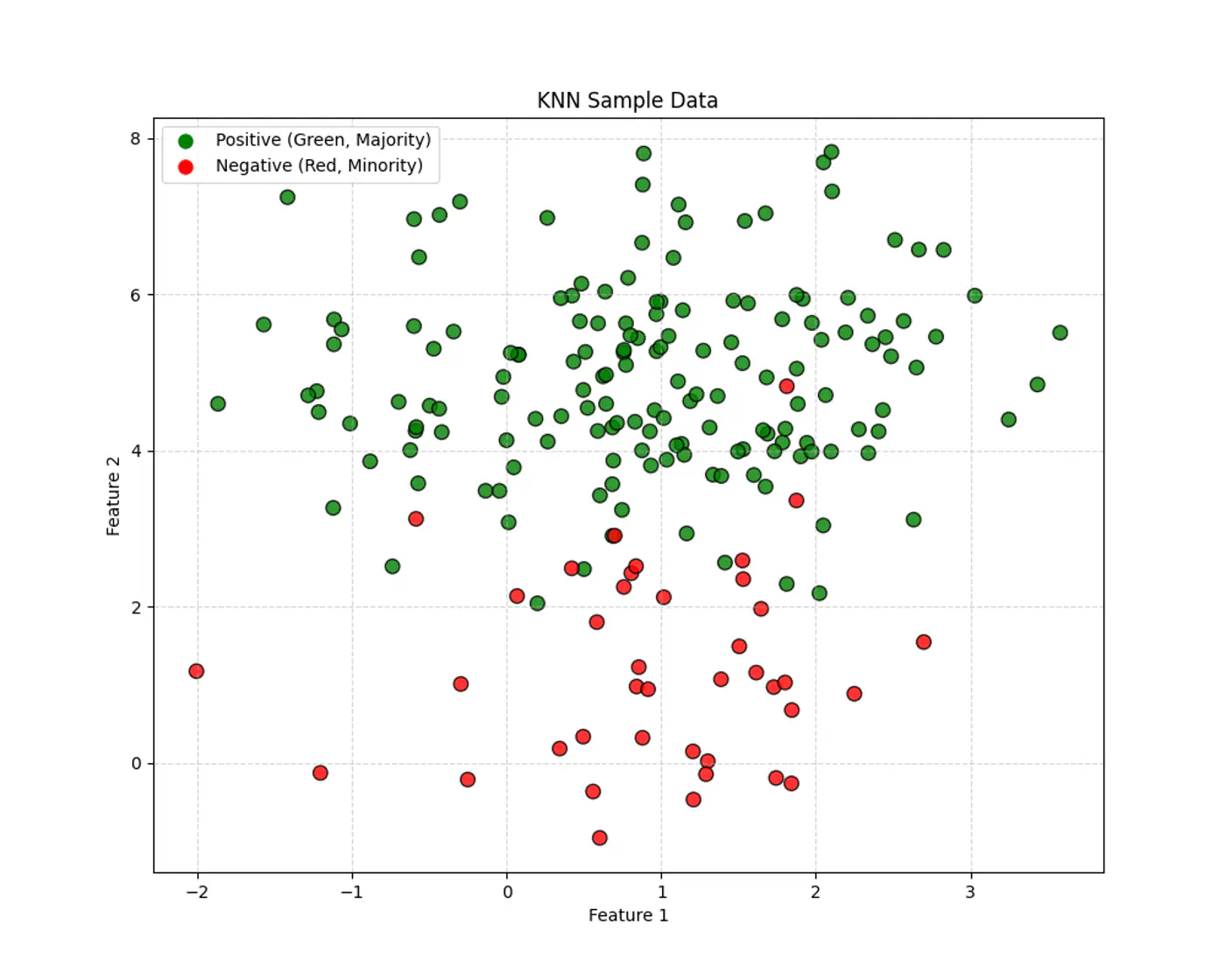
Let’s use this dataset to understand the impact of number of neighbours ‘k’.

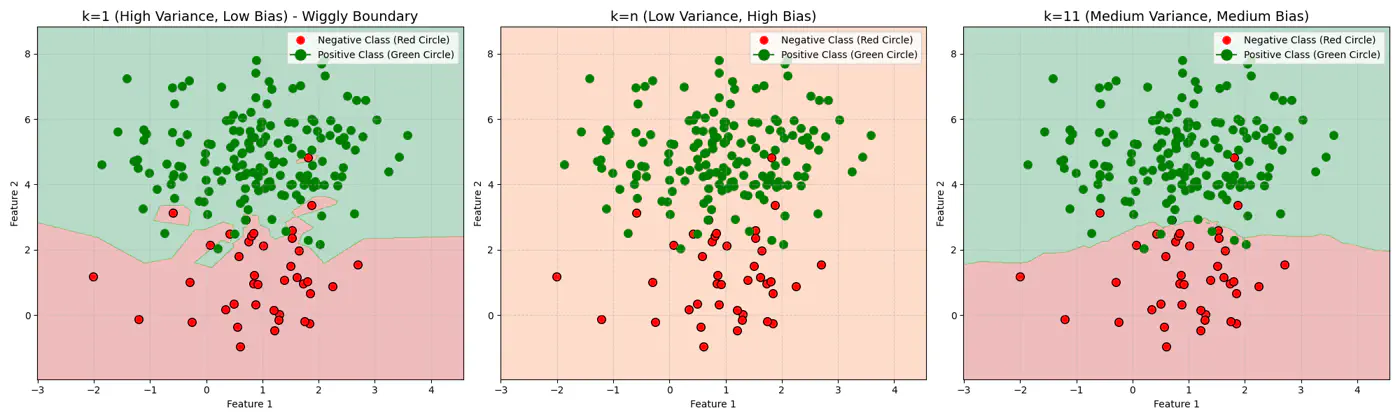
👉If ‘k’ is very large, say, k=n,

• model simply predicts the majority class of the entire dataset for every query point , i.e, under-fitting.

👉If ‘k’ is very small, say, k=1,

• model is highly sensitive to noise or outliers, as it looks at only 1 nearest neighbor, i.e, over-fitting.

Let’s plot Error vs ‘K’ neighbors:

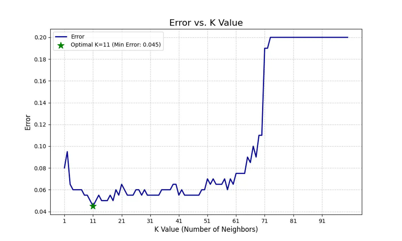
• Figure 1: k=1, Over-fitting

• Figure 2: k=n, Under-fitting

• Figure 3: k=11, Lowest Error (Optimum)