This is the multi-page printable view of this section. Click here to print.
K Nearest Neighbors
1 - KNN Introduction
- Parametric models:
- Rely on assumption that relationships between data points are linear.
- For polynomial regression we need to find the degree of polynomial.
- Training:
- We need to train the model for prediction.
Simple: Intuitive way to classify data or predict values by finding similar existing data points (neighbors).
Non-Parametric: Makes no assumptions about the underlying data distribution.
No Training Required: KNN is a ‘lazy learner’, it does not require a formal training phase.

Given a query point \(x_q\) and a dataset, D = {\((x_i,y_i)_{i=1}^n, \quad x_i,y_i \in \mathbb{R}^d\)}, the algorithm finds a set of ‘k’ nearest neighbors \(\mathcal{N}_k(x_q) \subseteq D\).
Inference:
- Choose a value of ‘k’ (hyper-parameter); odd number.
- Calculate distance (Euclidean, Cosine etc.) between and every point in dataset and store in a distance list.
- Sort the distance list in ascending order; choose top ‘k’ data points.
- Make prediction:
- Classification: Take majority vote of ‘k’ nearest neighbors and assign label.
- Regression: Take the mean/median of ‘k’ nearest neighbors.
Note: Store entire dataset.
- Storing Data: Space Complexity: O(nd)
- Inference: Time Complexity: O(nd + nlogn)
Explanation:
- Distance to all ’n’ points in ‘d’ dimensions: O(nd)
- Sorting all ’n’ data points : O(nlogn)
Note: Brute force KNN is unacceptable when ’n’ is very large, say billions.
2 - KNN Optimizations
Naive KNN needs some improvements to fix some of its drawbacks.
- Standardization
- Distance-Weighted KNN
- Mahalanobis Distance
Say one feature is ‘Annual Income’ (0-1M), and another feature is ‘Years of Experience’ (0-40).
The Euclidean distance will be almost entirely dominated by income .
So, we do standardization of each feature, such that it has a mean, \(\mu\)=0 and variance,\(\sigma\)=1.
\[z=\frac{x-\mu}{\sigma}\]Vanilla KNN treats the 1st nearest neighbor and the k-th nearest neighbor as equal.
A neighbor that is 0.1units away should have more influence than a neighbor that is 10 units away.
We assign weight to each neighbor; most common strategy is inverse of squared distance.
\[w_i = \frac{1}{d(x_q, x_i)^2 + \epsilon}\]Improvements:
- Noise/Outlier: Reduces the impact of ‘noise’ or ‘outlier’ (distant neighbors).
- Imbalanced Data: Closer points dominate, mitigating impact of imbalanced data.
- e.g: If you have a query point surrounded by 2 very close ‘Class A’ points and 3 distant ‘Class B’ points, weighted ️♀️ KNN will correctly pick ‘Class A'.
Problem
Euclidean distance makes assumption that all the features are independent and provide unique information.
‘Height’ and ‘Weight’ are highly correlated.
So, if we use Euclidean distance, we are effectively ‘double-counting’ the size of the person.
Mahalanobis distance measures distance in terms of standard deviations from the mean, accounting for the covariance between features.
\[d(x, y) = \sqrt{(x - y)^T \Sigma^{-1} (x - y)}\]\(\Sigma\): Covariance matrix of the data
- If \(\Sigma\) is identity matrix, Mahalanobis distance reduces to Euclidean distance.
- If \(\Sigma\) is a diagonal matrix, Mahalanobis distance reduces to Normalized Euclidean distance.
Naive KNN shifts all computation to inference time, and it is very slow.
- To find the neighbor for one query, we must touch every single bit of the ‘nxd’ matrix.
- If n=10^9,a single query would take seconds, but we need milliseconds.
- Distance Weighted KNN
- K-D Trees (d<20): Recursively partitions space into axis-aligned hyper-rectangles. O(log N ) search.
- Ball Trees : High dimensional data; Haversine distance for geospatial data.
- Approximate Nearest Neighbors (ANN)
- Locality Sensitive Hashing (LSH): Uses ‘bucketizing’ ️ hashes. Points that are close have a high probability of having the same hash.
- Hierarchical Navigable Small World (HNSW); Graph of vectors; Search is a ‘greedy walk’ across levels.
- Product Quantization (Reduce memory footprint of high dimensional vectors)
- ScaNN (Google)
- FAISS (Meta)
- Dimensionality Reduction (Mitigate ‘Curse of Dimensionality’)
- PCA
3 - Curse Of Dimensionality
While Euclidean distance(L norm) is the most frequently discussed, ‘Curse of Dimensionality’ impacts all Minkowski norms (\(L_p\))
\[L_p = (\sum |x_i|^p)^{\frac{1}{p}} \]Note: ‘Curse of Dimensionality’ is largely a function of the exponent (p) in the distance calculation.
Coined by mathematician John Bellman in the 1960s while studying dynamic programming.
High dimensional data created following challenges:
- Distance Concentration
- Data Sparsity
- Exponential Sample Requirement
Consider a hypercube in d-dimensions of side length = 1; Volume = \(1^d\) = 1
A smaller inner cube with side length = 1 - \(\epsilon\) ; Volume = \((1 -\epsilon)^d\)
This implies that almost all the volume of the high-dimensional cube lies near the ‘crust’.
e.g: if \(\epsilon\)= 0.01, d = 500; Volume of inner cube = \((1 -0.01)^{500}\) = \(0.99^{500}\) = 0.006 = 0.6%
Consequently, all points become nearly equidistant, and the concept of ‘nearest’ or ‘neighborhood’ loses
its meaning.
The volume of the feature space increases exponentially with each added dimension.
To maintain the same data density found in a 1D space with 10 points, we would need \(10^{10}\)(10 billion) points in 10D space.
Because real-world datasets are rarely this large, the data becomes “sparse” making it difficult to find truly similar neighbors.
To maintain a reliable result, the amount of training data needed must grow exponentially with the number of dimensions.
Without this growth, the model is highly prone to overfitting, where it learns from noise in the ‘sparse’ data
rather than actual underlying patterns.
Note: For modern embeddings (often 768 or 1536 dimensions), it is mathematically impossible to collect enough data to ‘fill’ the space.
- Cosine Similarity
- Normalization
Cosine similarity measures the cosine of the angle between 2 vectors.
\[\text{cos}(\theta) = \frac{A \cdot B}{\|A\|\|B\|} = \frac{\sum_{i=1}^{D} A_i B_i}{\sqrt{\sum_{i=1}^{D} A_i^2} \sqrt{\sum_{i=1}^{D} B_i^2}}\]Note: Cosine similarity mitigates the ‘curse of dimensionality" problem.
Normalize the vector, i.e, make its length =1, a unit vector.
By normalizing, we project all points onto the surface of a unit hypersphere.
- We are no longer searching in the ‘empty’ high-dimensional volume of a hypercube.
- Now, we are searching on a constrained manifold (the shell).
Note: By normalizing, we move the data from the volume of the D-dimensional space onto the surface of a (D-1)-dimensional hypersphere.
Euclidean Distance Squared of Normalized Vectors:
\[ \begin{align*} \|A - B\|^2 &= (A - B) \cdot (A - B) \\ &= \|A\|^2 + \|B\|^2 - 2(A \cdot B)\\ \because \|A\| &= \|B\| = 1 \\ \|A - B\|^2 &= 1 + 1 - 2\cos(\theta) \\ \therefore \|A - B\|^2 &= 2(1 - \cos(\theta))\\ \end{align*} \]Note: This formula proves that maximizing ‘Cosine similarity’ is identical to minimizing ‘Euclidean distance’ on the hypersphere.
4 - Bias Variance Tradeoff
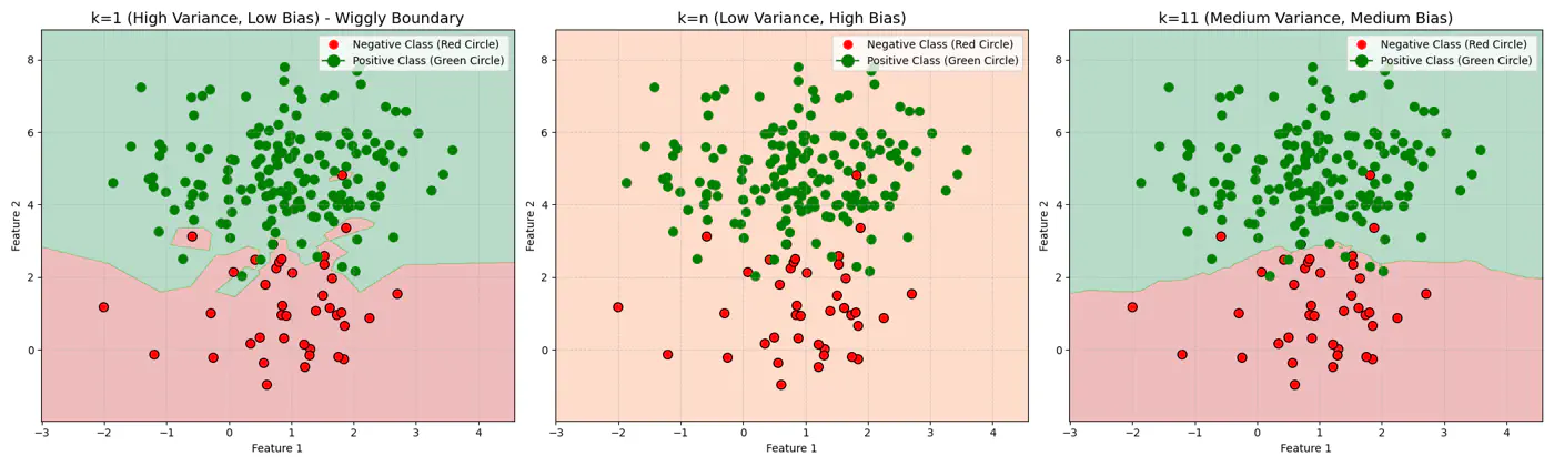
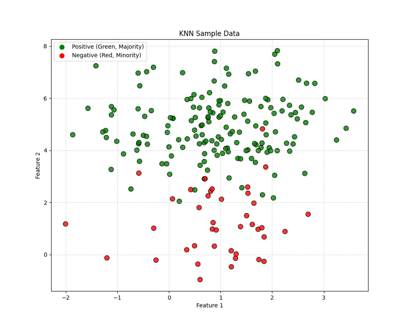
Let’s use this dataset to understand the impact of number of neighbours ‘k’.
If ‘k’ is very large, say, k=n,
- model simply predicts the majority class of the entire dataset for every query point , i.e, under-fitting.
If ‘k’ is very small, say, k=1,
- model is highly sensitive to noise or outliers, as it looks at only 1 nearest neighbor, i.e, over-fitting.
Let’s plot Error vs ‘K’ neighbors:
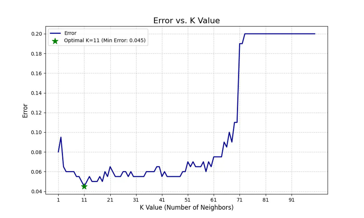
Figure 1: k=1, Over-fitting
Figure 2: k=n, Under-fitting
Figure 3: k=11, Lowest Error (Optimum)