This is the multi-page printable view of this section. Click here to print.
Linear Regression
1 - Meaning of 'Linear'
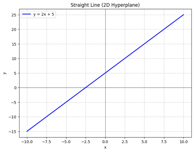
Equation of a line is of the form \(y = mx + c\).
To represent a line in 2D space, we need 2 things:
- m = slope or direction of the line
- c = y-intercept or distance from the origin
Similarly,
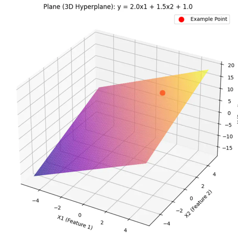
A hyperplane is a lower (d-1) dimensional sub-space that divides a d-dimensional space into 2 distinct parts.
Equation of a hyperplane:
Here, ‘y’ is expressed as a linear combination of parameters - \( w_0, w_1, w_2, \dots, w_n \)
Hence - Linear means the model is ‘linear’ with respect to its parameters NOT the variables.
Read more about Hyperplane
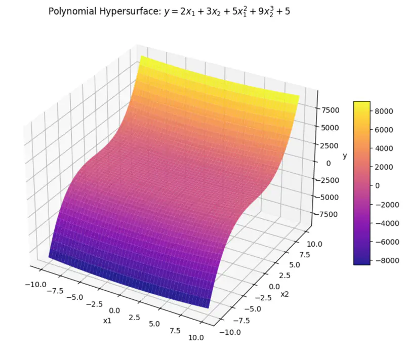
can be rewritten as:
\[y = w_1x_1 + w_2x_2 + w_3x_3 + w_4x_4 + w_0\]where, \(x_3 = x_1^2 ~ and ~ x_4 = x_2^3 \)
\(x_3 ~ and ~ x_4 \) are just 2 new (polynomial) variables.
And, ‘y’ is still a linear combination of parameters: \(w_0, w_1, \dots w_4\)
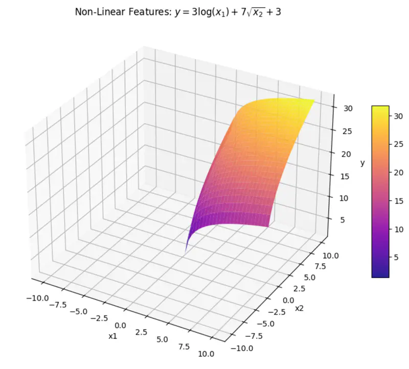
can be rewritten as:
\[y = w_1x_1 + w_2x_2 + w_0\]where, \(x_1 = log(x) ~ and ~ x_2 = \sqrt{x} \)
\(x_1 ~ and ~ x_2 \) are are transformations of variable \(x\).
And, ‘y’ is still a linear combination of parameters: \(w_0, w_1, ~and~ w_2\)
Even if we take log, we get:
\[log(y) = w_1log(x_1) + w_2log(x_2) + log(w_0)\]here, \(log(w_0) \) parameter is NOT linear.
End of Section
2 - Meaning of 'Regression'
Regression = Going Back
Regression has a very specific historical origin that is different from its current statistical meaning.
Sir Francis Galton (19th century), cousin of Charles Darwin, coined 🪙 this term.
Observation:
Galton observed that -
the children 👶 of unusually tall ⬆️ parents 🧑🧑🧒🧒,
tended to be shorter ⬇️ than their parents 🧑🧑🧒🧒,
and children 👶 of unusually short ⬇️ parents 🧑🧑🧒🧒,
tended to be taller ⬆️ than their parents 🧑🧑🧒🧒.
Galton named this biological tendency - ‘regression towards mediocrity/mean’.
Galton used method of least squares to model this relationship, by fitting a line to the data 📊.
Regression = Fitting a Line
Over time ⏳, the name ‘regression’ got permanently attached to the method of fitting line to the data 📊.
Today in statistics and machine learning, ‘regression’ universally refers to the method of finding the
‘line of best fit’ for a set of data points, NOT the concept of ‘regressing towards the mean’.
End of Section
3 - Linear Regression
Let’s understand linear regression using an example to predict salary.
Predict the salary 💰 of an IT employee, based on various factors, such as, years of experience, domain, role, etc.
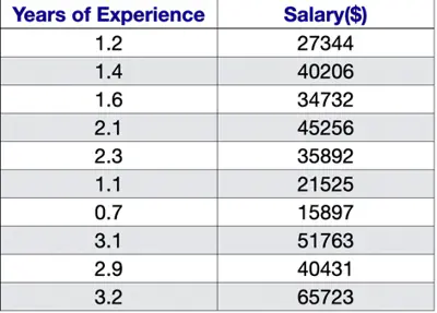
Let’s start with a simple problem and predict the salary using only one input feature.
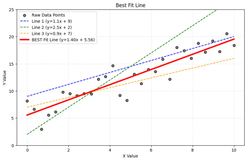
Goal 🎯 : Find the line of best fit.
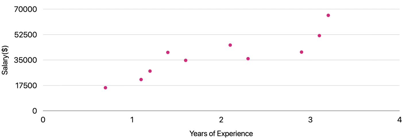
Plot: Salary vs Years of Experience
\[y = mx + c = w_1x + w_0\]Slope = \(m = w_1 \)
Intercept = \(c = w_0\)
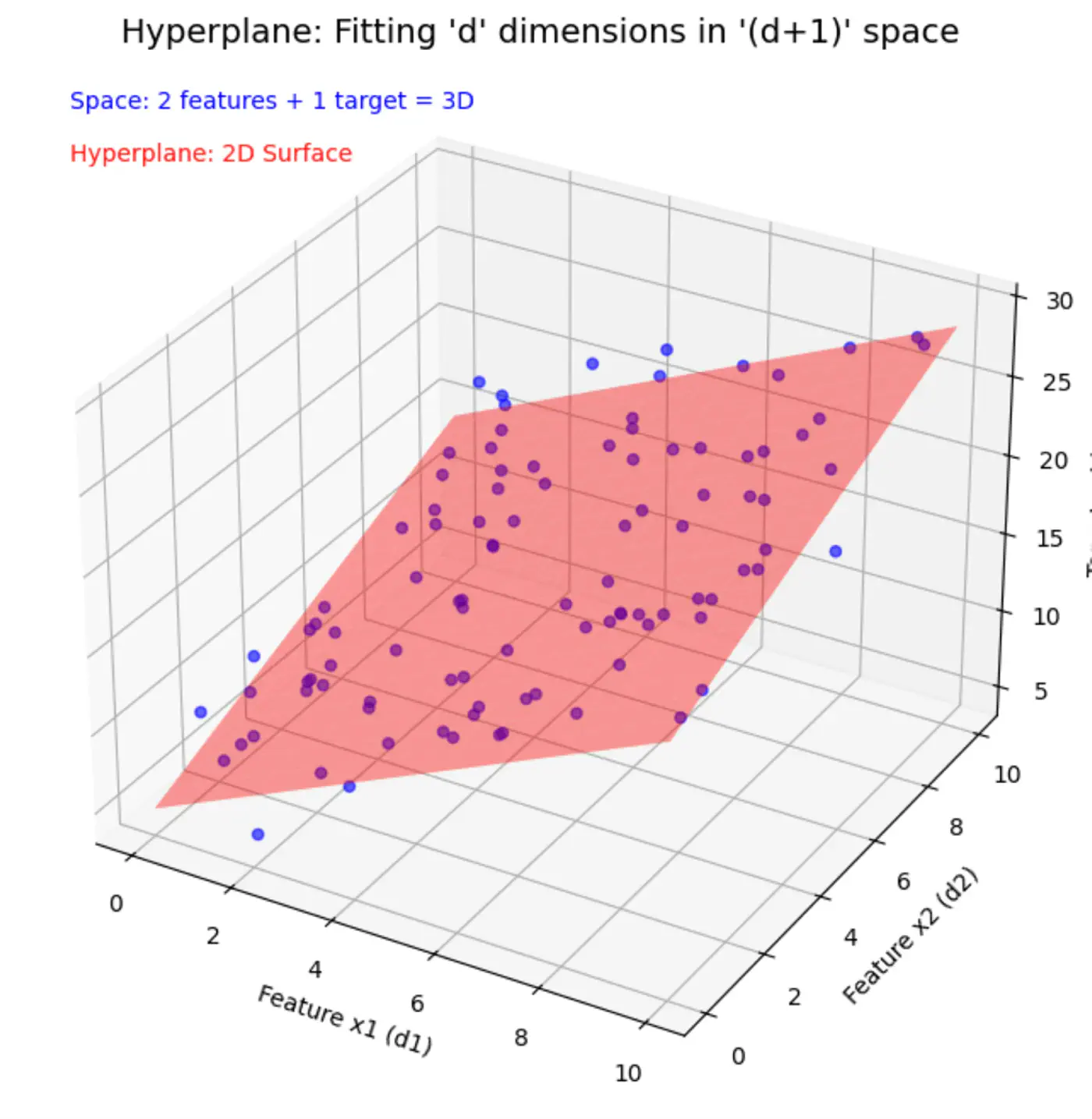
Similarly, if we include other factors/features impacting the salary 💰, such as, domain, role, etc, we get an equation of a fitting hyperplane:
\[y = w_1x_1 + w_2x_2 + \dots + w_dx_d + w_0\]where,
\[ \begin{align*} x_1 &= \text{Years of Experience} \\ x_2 &= \text{Domain (Tech, BFSI, Telecom, etc.)} \\ x_3 &= \text{Role (Dev, Tester, DevOps, ML, etc.)} \\ x_d &= d^{th} ~ feature \\ w_0 &= \text{Salary of 0 years experience} \\ \end{align*} \]Space = ’d’ features + 1 target variable = ’d+1’ dimensions
In a ’d+1’ dimensional space, we try to fit a ’d’ dimensional hyperplane.
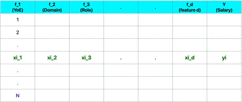
Let, data = \( {(x_i, y_i)}_{i=1}^N ; ~ x_i \in R^d , y_i \in R^d\)
where, N = number of training samples.
Note: Fitting hyperplane (\(y = w_1x_1 + w_2x_2 + \dots + w_dx_d + w_0\)) is the model.
Objective 🎯: find the parameters/weights (\(w_0, w_1, w_2, \dots w_d \)) of the model.
\(\mathbf{w} = \begin{bmatrix} w_1 \\ w_2 \\ \vdots \\ w_d \end{bmatrix}_{\text{d x 1}}\)
\( \mathbf{x_i} = \begin{bmatrix} x_{i_1} \\ x_{i_2} \\ \vdots \\ x_{i_d} \end{bmatrix}_{\text{d x 1}} \)
\( \mathbf{y} = \begin{bmatrix} y_1 \\ y_2 \\ \vdots \\ y_i \\ \vdots \\ y_n \end{bmatrix}_{\text{n x 1}} \)
\( X =
\begin{bmatrix}
x_{11} & x_{12} & \cdots & x_{1d} \\
x_{21} & x_{22} & \cdots & x_{2d} \\
\vdots & \vdots & \ddots & \vdots \\
x_{i1} & x_{i2} & \cdots & x_{id} \\
\vdots & \vdots & \ddots & \vdots \\
x_{n1} & x_{n2} & \cdots & x_{nd} \\
\end{bmatrix}
_{\text{n x d}}
\)
Prediction:
Error = Actual - Predicted
\[ \epsilon_i = y_i - \hat{y_i}\]Goal 🎯: Minimize error between actual and predicted.
We can quantify the error for a single data point in following ways:
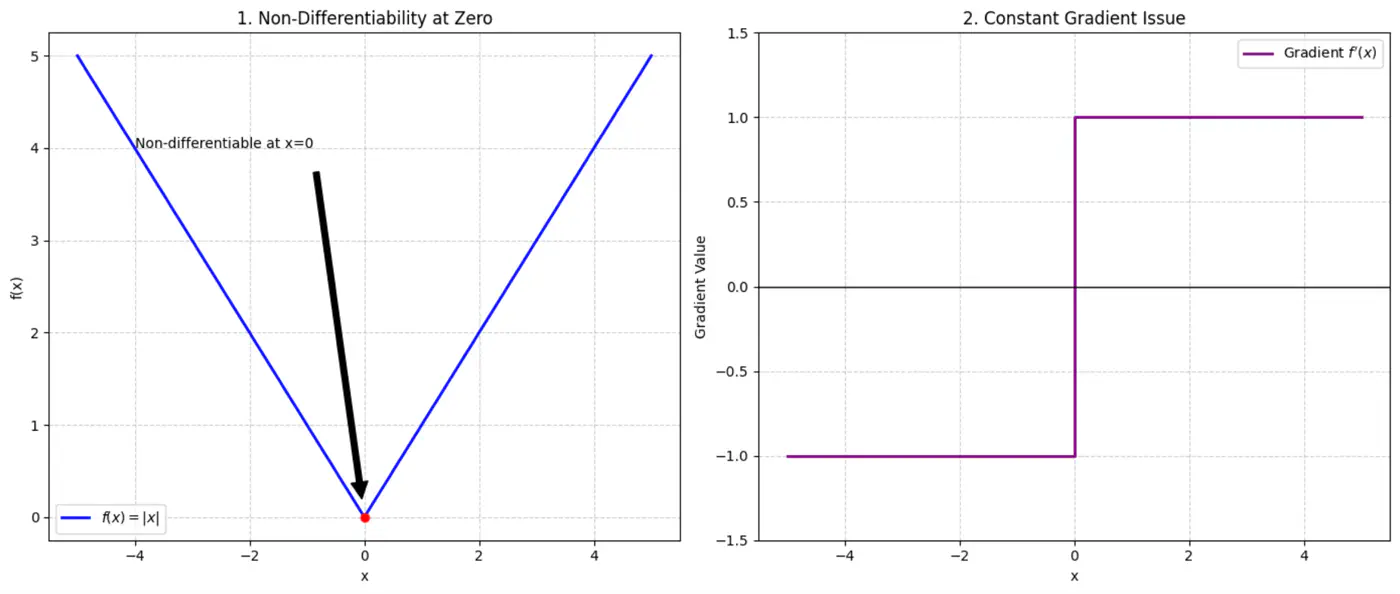
- Absolute error = \(|y_i - \hat{y_i}|\)
- Squared error = \((y_i - \hat{y_i})^2\)
Not differentiable at x=0, required for gradient descent.
Constant gradient, i.e \(\pm 1\), model learns at same rate, whether the error is large or small.
Average loss across all data points.
Mean Squared Error (MSE) =
\[ J(w) = \frac{1}{n} \sum_{i=1}^N (y_i - \hat{y_i})^2 \]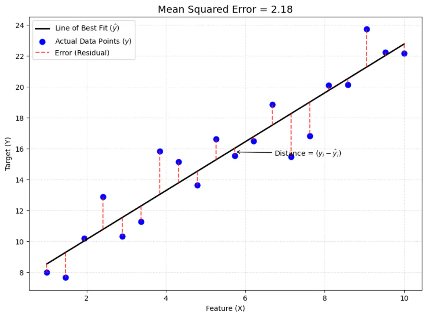
The above equation is quadratic in \(w_0, w_1, w_2, \dots w_d \).
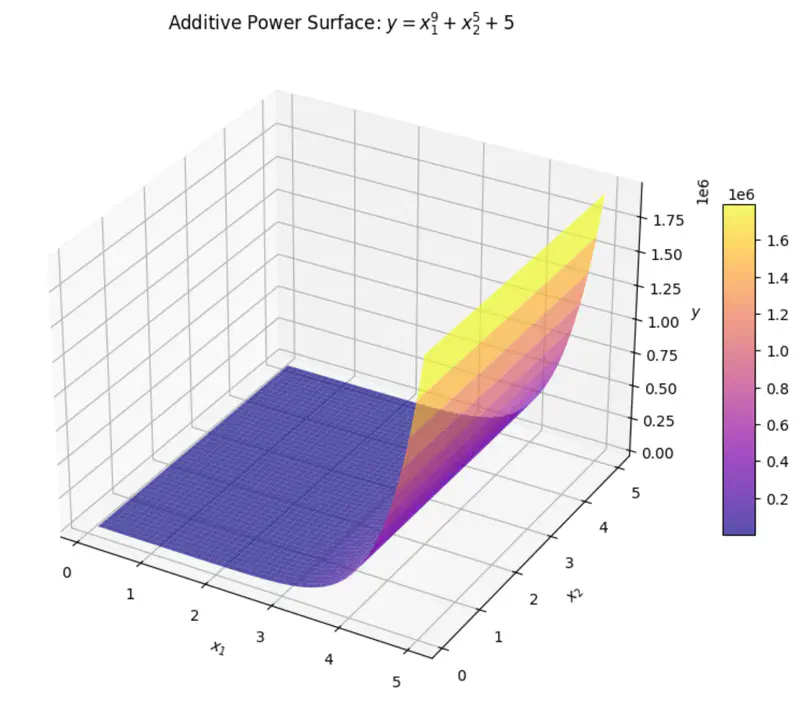
Below is an image of a Paraboloid in 3D, similarly we will have a Paraboloid in ’d’ dimensions.
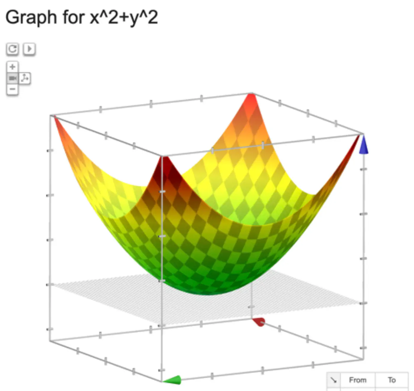
In order to find the minima of the cost function we need to take its derivative w.r.t weights and equate to 0.
\[ \begin{align*} \frac{\partial{J(w)}}{\partial{w_0}} = 0 \\ \frac{\partial{J(w)}}{\partial{w_1}} = 0 \\ \frac{\partial{J(w)}}{\partial{w_2}} = 0 \\ \vdots \\ \frac{\partial{J(w)}}{\partial{w_d}} = 0 \\ \end{align*} \]We have ‘d+1’ linear equations to solve for ‘d+1’ weights \(w_0, w_1, w_2, \dots , w_d\).
But solving ‘d+1’ system of linear equations (called the ’normal equations’) is tedious and NOT used for practical purposes.
where,
\(\mathbf{w} = \begin{bmatrix} w_1 \\ w_2 \\ \vdots \\ w_d \end{bmatrix}_{\text{d x 1}}\)
\( \mathbf{x_i} = \begin{bmatrix} x_{i_1} \\ x_{i_2} \\ \vdots \\ x_{i_d} \end{bmatrix}_{\text{d x 1}} \)
\( \mathbf{y} = \begin{bmatrix} y_1 \\ y_2 \\ \vdots \\ y_i \\ \vdots \\ y_n \end{bmatrix}_{\text{n x 1}} \)
\( X =
\begin{bmatrix}
x_{11} & x_{12} & \cdots & x_{1d} \\
x_{21} & x_{22} & \cdots & x_{2d} \\
\vdots & \vdots & \ddots & \vdots \\
x_{i1} & x_{i2} & \cdots & x_{id} \\
\vdots & \vdots & \ddots & \vdots \\
x_{n1} & x_{n2} & \cdots & x_{nd} \\
\end{bmatrix}
_{\text{n x d}}
\)
Prediction:
Let’s expand the cost function J(w):
\[ \begin{align*} J(w) &= \frac{1}{n} (y - Xw)^2 \\ &= \frac{1}{n} (y - Xw)^T(y - Xw) \\ &= \frac{1}{n} (y^T - w^TX^T)(y - Xw) \\ J(w) &= \frac{1}{n} (y^Ty - w^TX^Ty - y^TXw + w^TX^TXw) \end{align*} \]Since,\(w^TX^Ty\), is a scalar, so it is equal to its transpose.
\[ w^TX^Ty = (w^TX^Ty)^T = y^TXw\]\[ J(w) = \frac{1}{n} (y^Ty - y^TXw - y^TXw + w^TX^TXw)\]\[ J(w) = \frac{1}{n} (y^Ty - 2y^TXw + w^TX^TXw) \]Note: \(X^2 = X^TX\) and \((AB)^T = B^TA^T\)
To find the minimum, take the derivative of cost function J(w) w.r.t ‘w’, and equate to 0 vector.
\[\frac{\partial{J(w)}}{\partial{w}} = \vec{0}\]\[ \begin{align*} &\frac{\partial{[\frac{1}{n} (y^Ty - 2y^TXw + w^TX^TXw)]}}{\partial{w}} = 0\\ & \implies 0 - 2X^Ty + (X^TX + X^TX)w = 0 \\ & \implies \cancel{2}X^TXw = \cancel{2} X^Ty \\ & \therefore \mathbf{w} = (X^TX)^{-1}X^T\mathbf{y} \end{align*} \]Note: \(\frac{\partial{(a^T\mathbf{x})}}{\partial{\mathbf{x}}} = a\) and \(\frac{\partial{(\mathbf{x}^TA\mathbf{x})}}{\partial{\mathbf{x}}} = (A + A^T)\mathbf{x}\)
This is the closed-form solution of normal equations.
- Inverse may NOT exist (non-invertible).
- Time complexity of calculating the inverse is O(n^3).
If the inverse does NOT exist then we can use the approximation of the inverse, also called Pseudo Inverse or Moore Penrose Inverse (\(A^+\)).
Moore Penrose Inverse ( \(A^+\)) is calculated using Singular Value Decomposition (SVD).
SVD of \(A = U \Sigma V^T\)
Pseudo Inverse \(A^+ = V \Sigma^+ U^T\)
Where, \(\Sigma^+\) is a transpose of \(\Sigma\) with reciprocals of non-zero singular values on its diagonals.
e.g:
Note: Time Complexity = O(mn^2)
End of Section
4 - Probabilistic Interpretation
Error = Random Noise, Un-modeled effects
\[ \begin{align*} \epsilon_i = y_i - \hat{y_i} \\ \implies y_i = \hat{y_i} + \epsilon_i \\ \because \hat{y_i} = x_i^Tw \\ \therefore y_i = x_i^Tw + \epsilon_i \\ \end{align*} \]Actual value(\(y_i\)) = Deterministic linear predictor(\(x_i^Tw\)) + Error term(\(\epsilon_i\))
- Independent and Identically Distributed (I.I.D):
Each error term is independent of others. - Normal (Gaussian) Distributed:
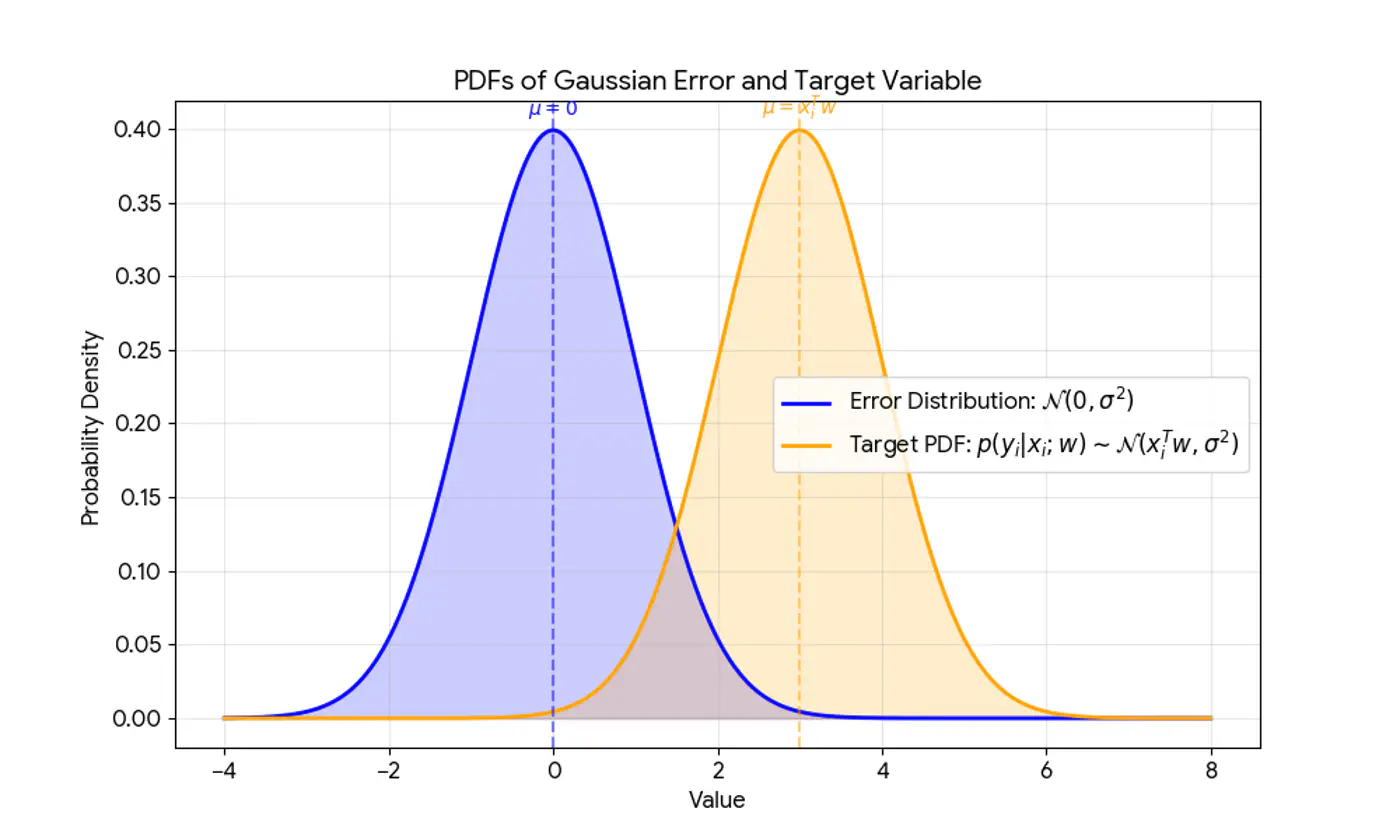
Error follows a normal distribution with mean = 0 and a constant variance, .
This implies that the target variable itself is a random variable, normally distributed around the linear relationship.
\[(y_{i}|x_{i};w)∼N(x_{i}^{T}w,\sigma^{2})\]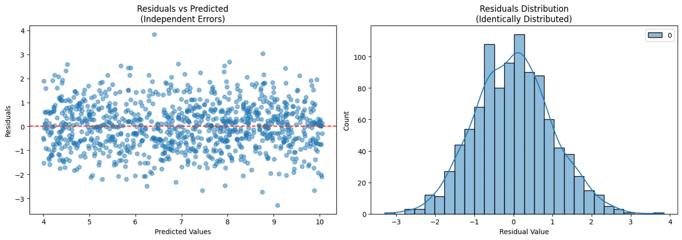
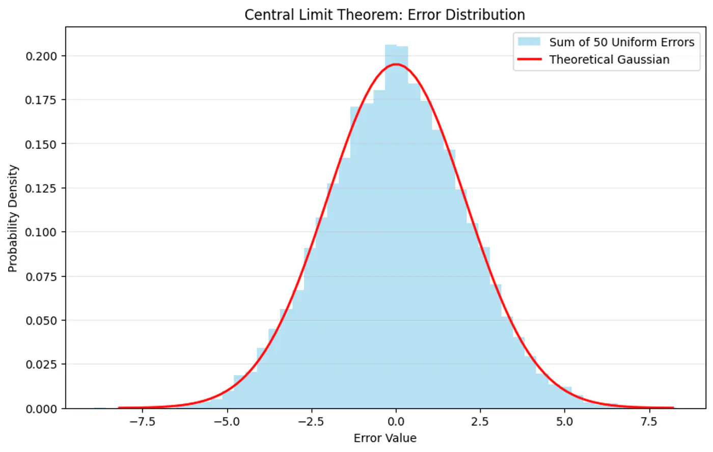
Central Limit Theorem (CLT) states that for a sequence of I.I.D random variables, the distribution of the sample mean(sum) approximates to a normal distribution, regardless of the original population distribution.
- Probability (Forward View):
Quantifies the chance of observing a specific outcome given a known, fixed model. - Likelihood (Backward/Inverse View):
Inverse concept used for inference (working backward from results to causes). It is a function of the parameters and measures how ‘likely’ a specific set of parameters makes the observed data appear.
‘Find the most plausible explanation for what I see.'
The goal of the probabilistic interpretation is to find the parameters ‘w’ that maximize the probability (likelihood) of observing the given dataset.
Assumption: Training data is I.I.D.
\[ \begin{align*} Likelihood &= \mathcal{L}(w) \\ \mathcal{L}(w) &= p(y|x;w) \\ &= \prod_{i=1}^N p(y_i| x_i; w) \\ &= \prod_{i=1}^N \frac{1}{\sigma\sqrt{2\pi}}e^{-\frac{(y_i-x_i^Tw)^2}{2\sigma^2}} \end{align*} \]Maximizing the likelihood function is mathematically complex due to the product term and the exponential function.
A common simplification is to maximize the log-likelihood function instead, which converts the product into a sum.
Note: Log is a strictly monotonically increasing function.
Note: The first term is constant w.r.t ‘w'.
So, we need to find parameters ‘w’ that maximize the log likelihood.
\[ \begin{align*} log \mathcal{L}(w) & \propto -\frac{1}{2\sigma^2} \sum_{i=1}^N (y_i-x_i^Tw)^2 \\ & \because \frac{1}{2\sigma^2} \text{ is constant} \\ log \mathcal{L}(w) & \propto -\sum_{i=1}^N (y_i-x_i^Tw)^2 \\ \end{align*} \]Maximizing the log-likelihood is equivalent to minimizing the sum of squared errors, which is the exact objective of the ordinary least squares (OLS) method.
\[ \underset{w}{\mathrm{min}}\ J(w) = \underset{w}{\mathrm{min}}\ \sum_{i=1}^N (y_i - x_i^Tw)^2 \]End of Section
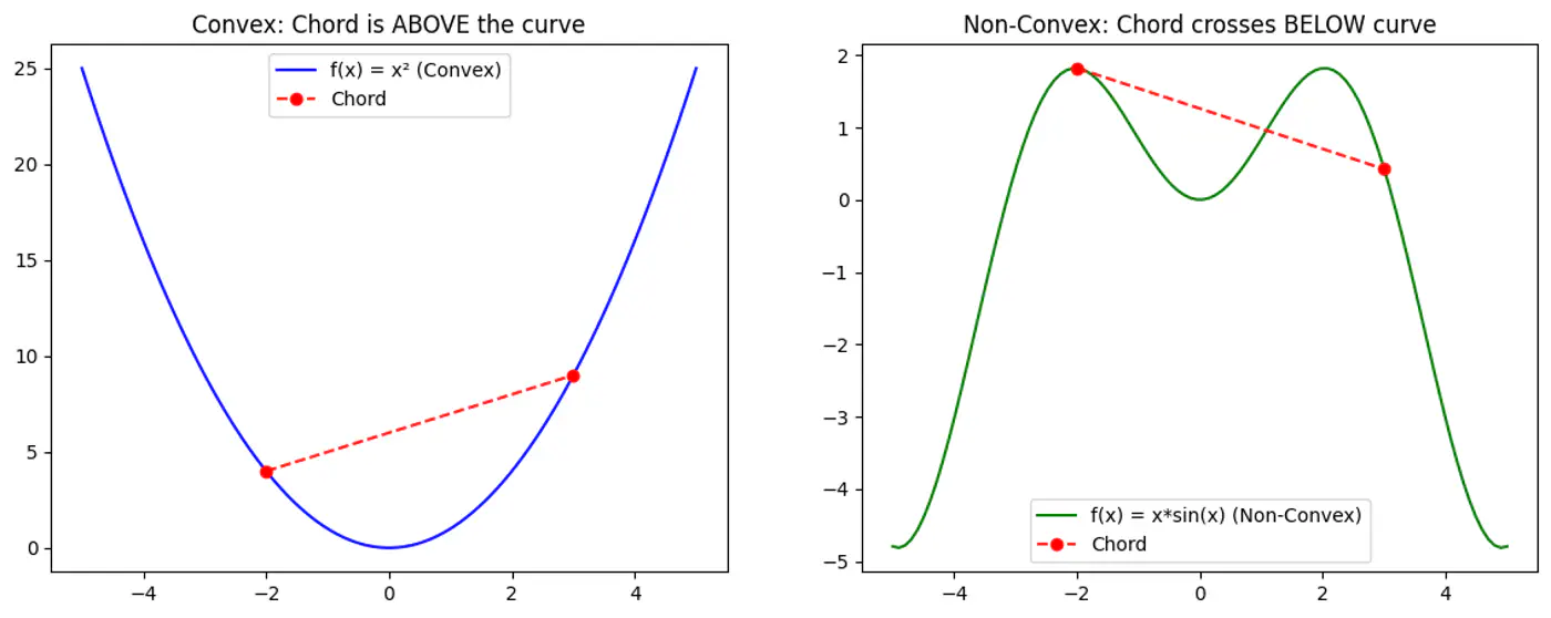
5 - Convex Function
Refers to a property of a function where a line segment connecting any two points on its graph lies above or on the graph itself.
A convex function is curved upwards.
MSE cost function J(w) is convex because its Hessian (H) is always positive semi definite.
\[\nabla J(\mathbf{w})=\frac{1}{n}\mathbf{X}^{T}(\mathbf{Xw}-\mathbf{y})\]\[\mathbf{H}=\frac{\partial (\nabla J(\mathbf{w}))}{\partial \mathbf{w}^{T}}=\frac{1}{n}\mathbf{X}^{T}\mathbf{X}\]\[\therefore \mathbf{H} = \nabla^2J(w) = \frac{1}{n} \mathbf{X}^{T}\mathbf{X}\]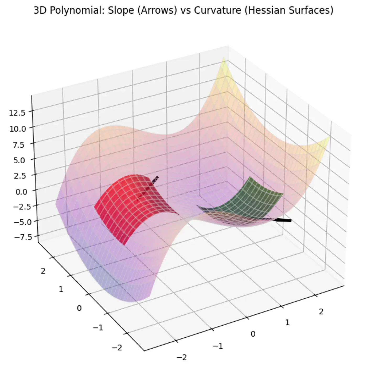
A matrix H is positive semi-definite if and only if for any non-zero vector ‘z’, the quadratic form \(z^THz \ge 0\).
For the Hessian of J(w),
\[ z^THz = z^T(\frac{1}{n}X^TX)z = \frac{1}{n}(Xz)^T(Xz) \]\((Xz)^T(Xz) = \lVert Xz \rVert^2\) = squared L2 norm (magnitude) of the vector
Note: The squared norm of any real-valued vector is always \(\ge 0\).
End of Section
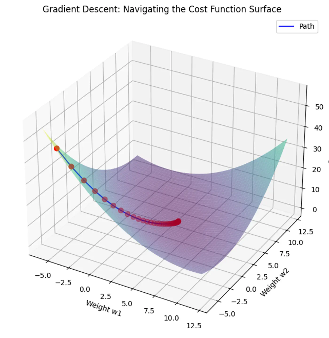
6 - Gradient Descent
Minimize the cost 💰function.
\[J(w)=\frac{1}{2n}(y-Xw)^{2}\]Note: The 1/2 term is included simply to make the derivative cleaner (it cancels out the 2 from the square).
Normal Equation (Closed-form solution) jumps straight to the optimal point in one step.
\[w=(X^{T}X)^{-1}X^{T}y\]But it is not always feasible and computationally expensive 💰(due to inverse calculation 🧮)
An iterative optimization algorithm slowly nudges parameters ‘w’ towards a value that minimize the cost💰 function.
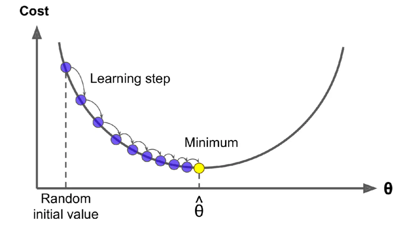
- Initialize the weights/parameters with random values.
- Calculate the gradient of the cost function at current parameter values.
- Update the parameters using the gradient. \[ w_{new} = w_{old} - \eta \frac{\partial{J(w)}}{\partial{w_{old}}} \] \( \eta \) = learning rate or step size to take for each parameter update.
- Repeat 🔁 steps 2 and 3 iteratively until convergence (to minima).
Applying chain rule:
\[ \begin{align*} &\text{Let } u = (y - Xw) \\ &\text{Derivative of } u^2 \text{ w.r.t 'w' }= 2u.\frac{\partial{u}}{\partial{w}} \\ \frac{\partial{(\frac{1}{2n} (y - Xw)^2)}}{\partial{w}} &= \frac{1}{\cancel2n}.\cancel2(y - Xw).\frac{\partial{(y - Xw)}}{\partial{w}} \\ &= \frac{1}{n}(y - Xw).X^T.(-1) \\ \therefore \frac{\partial{J(w)}}{\partial{w}} &= \frac{1}{n}X^T(Xw - y) \end{align*} \]Note: \(\frac{∂(a^{T}x)}{∂x}=a\)
Update parameter using gradient:
\[ w_{new} = w_{old} - \eta'. X^T(Xw - y) \]- Most important hyper parameter of gradient descent.
- Dictates the size of the steps taken down the cost function surface.
Small \(\eta\) ->
Large \(\eta\) ->
- Learning Rate Schedule:
The learning rate is decayed (reduced) over time.
Large steps initially and fine-tuning near the minimum, e.g., step decay or exponential decay. - Adaptive Learning Rate Methods:
Automatically adjust the learning rate for each parameter ‘w’ based on the history of gradients.
Preferred in modern deep learning as they require less manual tuning, e.g., Adagrad, RMSprop, and Adam.
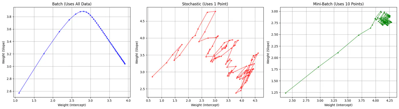
Batch, Stochastic, Mini-Batch are classified by data usage for gradient calculation in each iteration.
- Batch Gradient Descent (BGD): Entire Dataset
- Stochastic Gradient Descent (SGD): Random Point
- Mini-Batch Gradient Descent (MBGD): Subset
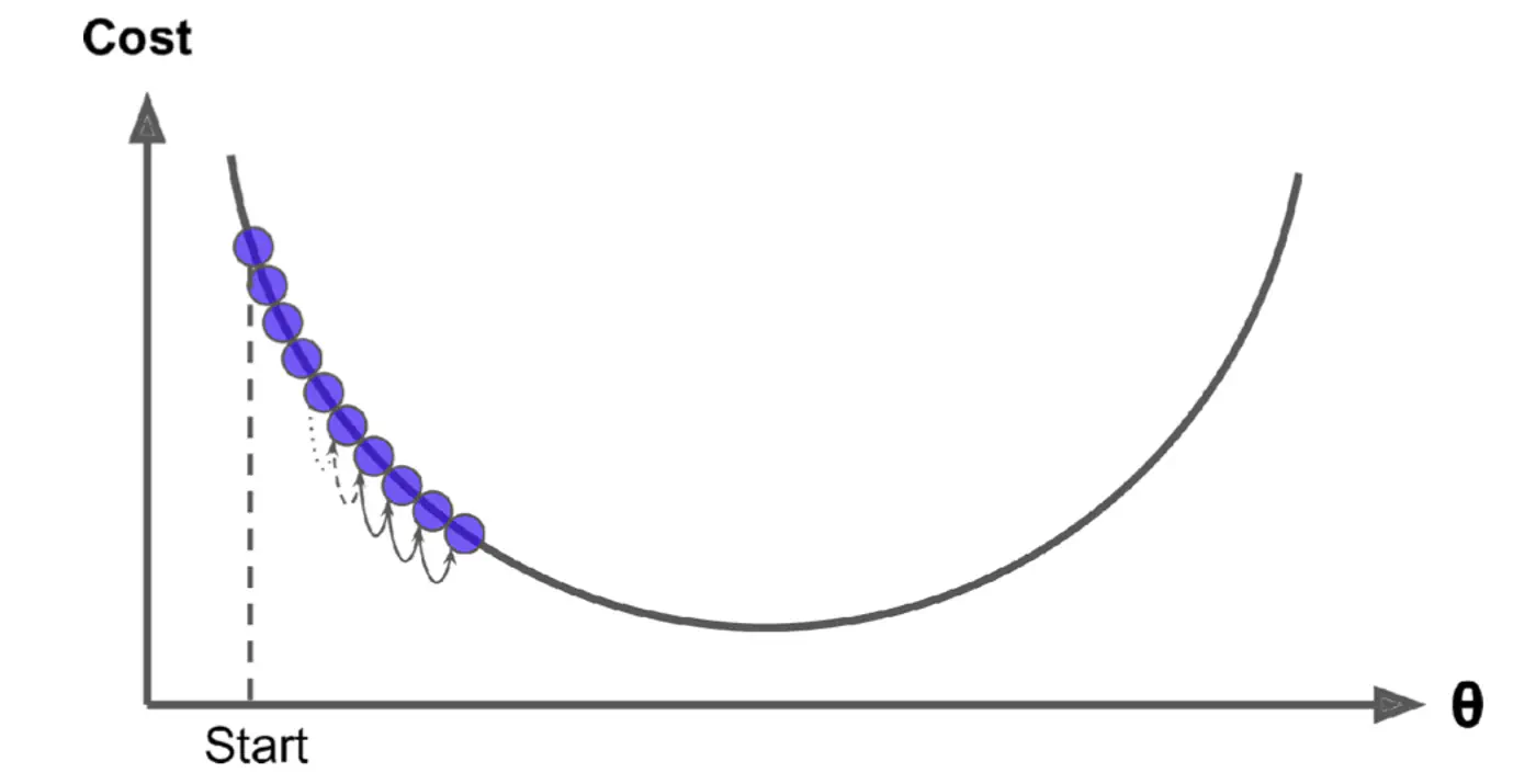
Computes the gradient using all the data points in the dataset for parameter update in each iteration.
\[w_{new} = w_{old} - \eta.\text{(average of all ’n’ gradients)}\]🔑Key Points:
- Slow 🐢 steps towards convergence, i.e, TC = O(n).
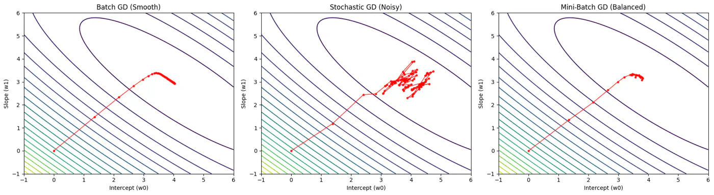
- Smooth, direct path towards minima.
- Minimum number of steps/iterations.
- Not suitable for large datasets; impractical for Deep Learning, as n = millions/billions.
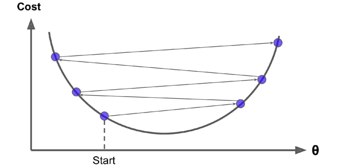
Uses only 1 data point selected randomly from dataset to compute gradient for parameter update in each iteration.
\[w_{new} = w_{old} - \eta.\text{(gradient at any random data point)}\]🔑Key Points:
- Computationally fastest 🐇 per step; TC = O(1).
- Highly noisy, zig-zag path to minima.
- High variance in gradient estimation makes path to minima volatile, requiring a careful decay of learning rate to ensure convergence to minima.
- Uses small randomly selected subsets of dataset, called mini-batch, (1<k<n), to compute gradient for parameter update in each iteration. \[w_{new} = w_{old} - \eta.\text{(average gradient of ‘k' data points)}\]
🔑Key Points:
- Moderate time ⏰ consumption per step; TC = O(k<n).
- Less noisy, and more reliable convergence than stochastic gradient descent.
- More efficient and faster than batch gradient descent.
- Standard optimization algorithm for Deep Learning.Note: Vectorization on GPUs allows for parallel processing of mini-batches; also GPUs are the reason for the mini-batch size to be a power of 2.
End of Section
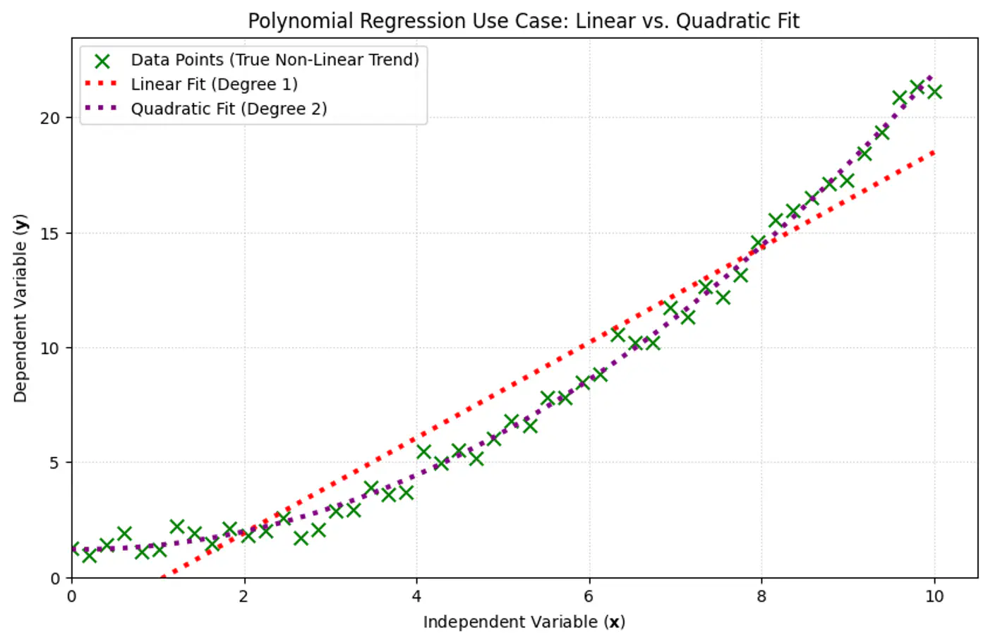
7 - Polynomial Regression
We can use a linear model to fit non-linear data.
Add powers of each feature as new features, then train a linear model on this extended set of features.
Linear: \(\hat{y_i} = w_0 + w_1x_{i_1} \)
Polynomial (quadratic): \(\hat{y_i} = w_0 + w_1x_{i_1} + w_2x_{i_1}^2\)
Polynomial (n-degree): \(\hat{y_i} = w_0 + w_1x_{i_1} + w_2x_{i_1}^2 +w_3x_{i_1}^3 + \dots + w_nx_{i_1}^n \)
Above polynomial can be re-written as linear equation:
\[\hat{y_i} = w_0 + w_1X_1 + w_2X_2 +w_3X_3 + \dots + w_nX_n \]where, \(X_1 = x_{i_1}, X_2 = x_{i_1}^2, X_3 = x_{i_1}^3, \dots, X_n = x_{i_1}^n\)
=> the model is still linear w.r.t to its parameters/weights \(w_0, w_1, w_2, \dots , w_n \).
e.g:
- Fit a linear model to the data points.
- Plot the errors.
- If the variance of errors is too high, then try polynomial features.
Note: Detect and remove outliers from error distribution.

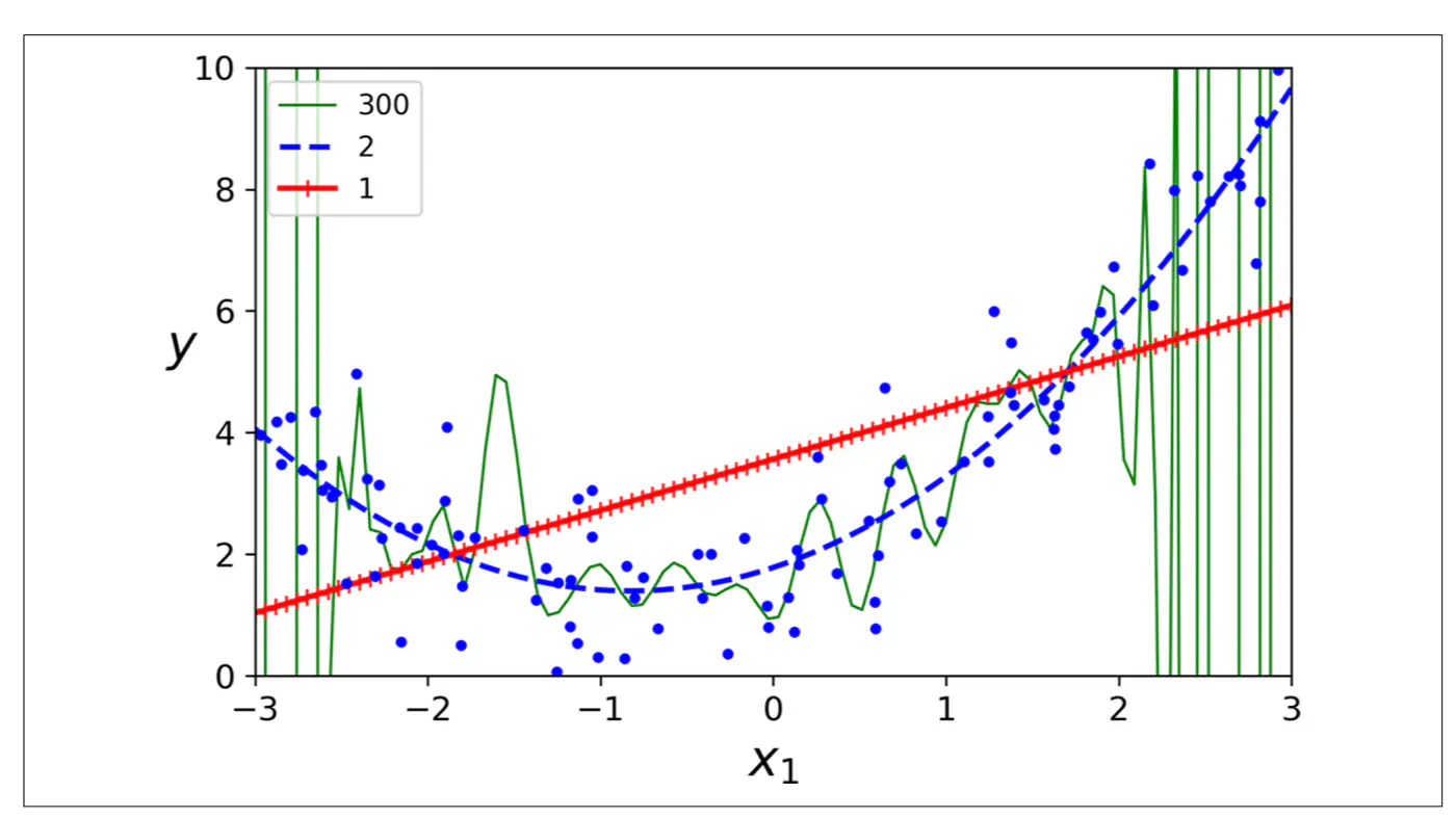
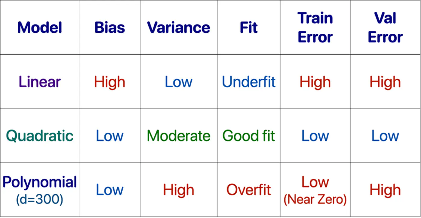
- Polynomial model : Over-fitting ❌
- Linear model : Under-fitting ❌
- Quadratic model: Generalizes best ✅
End of Section
8 - Data Splitting
- Training Data: Learn model parameters (Textbook + Practice problems)
- Validation Data: Tune hyper-parameters (Mock tests)
- Test Data: Evaluate model performance (Real (final) exam)
Data leakage occurs when information from the validation or test set is inadvertently used to train 🏃♂️ the model.
The model ‘cheats’ by learning to exploit information it should not have access to, resulting in artificially inflated performance metrics during testing 🧪.
- Small datasets(1K-100K): 60/20/20, 70/15/15 or 80/10/10
- Large datasets(>1M): 98/1/1 would suffice, as 1% of 1M is still 10K.
Note: There is no fixed rule, its trial and error.
If there is class imbalance in the dataset, (e.g., 95% class A , 5% class B), a random split might result in the validation set having 99% class A.
Solution: Use stratified sampling to ensure class proportions are maintained across all splits (train️/validation/test).
Note: Non-negotiable for imbalanced data.
- In time-series ⏰ data, divide the data chronologically, not randomly, i.e, training data time ⏰ should precede validation data time ⏰.
- We always train 🏃♂️ on past data to predict future data.
Golden rule: Never look 👀 into the future.
End of Section
9 - Cross Validation
Do not trust one split of the data; validate across many splits, and average the result to reduce randomness and bias.
Note: Two different splits of the same dataset can give very different validation scores.
Cross-validation is a statistical resampling technique used to evaluate how well a machine learning model generalizes to an independent, unseen dataset.
It works by systematically partitioning the available data into multiple subsets, or ‘folds’, and then training and testing the model on different combinations of these folds.
- K-Fold Cross-Validation
- Leave-One-Out Cross-Validation (LOOCV)
- Shuffle the dataset randomly (except time-series ⏳).
- Split data into k equal subsets(folds).
- Iterate through each unique fold, using it as the validation set.
- Use remaining k-1 fold for training 🏃♂️.
- Take an average of the results.Note: Common choice for k=5 or 10.
- Iteration 1: [V][T][T][T][T]
- Iteration 2: [T][V][T][T][T]
- Iteration 3: [T][T][V][T][T]
- Iteration 4: [T][T][T][V][T]
- Iteration 5: [T][T][T][T][V]
Model is trained 🏃♂️on all data points except one, and then tested 🧪on that remaining single observation.
LOOCV is an extreme case of k-fold cross-validation, where, k=n (number of data points).
Pros:
Useful for small (<1000) datasets.Cons:
Computationally 💻 expensive 💰.
End of Section
10 - Bias Variance Tradeoff
Mean Squared Error (MSE) = \(\frac{1}{n} \sum_{i=1}^n (y_i - \hat{y_i})^2\)
Total Error = Bias^2 + Variance + Irreducible Error
- Bias = Systematic Error
- Bias measures how far the average prediction of a model is from the true value.
- Variance = Sensitivity to Data
- Variance measures how much the predictions of a model vary for different training datasets.
- Irreducible Error = Sensor noise, Human randomness
- Inherent uncertainty in the data generation process itself and cannot be reduced by any model.
Systematic error from overly simplistic assumptions or strong opinion in the model.
e.g. House 🏠 prices 💰 = Rs. 10,000 * Area (sq. ft).
Note: This is over simplified view, because it ignores, amenities, location, age, etc.
Error from sensitivity to small fluctuations 📈 in the data.
e.g. Deep neural 🧠 network trained on a small dataset.
Note: Memorizes everything, including noise.
Say a house 🏠 in XYZ street was sold for very low price 💰.
Reason: Distress selling (outlier), or incorrect entry (noise).
Note: Model will make wrong(lower) price 💰predictions for all houses in XYZ street.
Goal 🎯 is to minimize total error.
Find a sweet-spot balance ⚖️ between Bias and Variance.
A good model ‘generalizes’ well, i.e.,
- Is not too simple or has a strong opinion.
- Does not memorize 🧠 everything in the data, including noise.
- Make model more complex.
- Add more features, add polynomial features.
- Decrease Regularization.
- Train 🏃♂️longer, the model has not yet converged.
- Add more data (most effective).
- Harder to memorize 🧠 1 million examples than 100.
- Use data augmentation, if getting more data is difficult.
- Increase Regularization.
- Early stopping 🛑, prevents memorization 🧠.
- Dropout (DL), randomly kill neurons, prevents co-adaptation.
- Use Ensembles.
- Averaging reduces variance.
Note: Co-adaptation refers to a phenomenon where neurons in a neural network become highly dependent on each other to detect features, rather than learning independently.
End of Section
11 - Regularization
Over-Fitting happens when we have a complex model that creates highly erratic curve to fit every single data point, including the random noise.
- Excellent performance on training 🏃♂️ data, but poor performance on unseen data.
- Penalty for overly complex models, i.e, models with excessively large or numerous parameters.
- Focus on learning general patterns rather than memorizing 🧠 everything, including noise in training 🏃♂️data.
Set of techniques that prevents over-fitting by adding a penalty term to the model’s loss function.
\[ J_{reg}(w) = J(w) + \lambda.\text{Penalty(w)} \]\(\lambda\) = Regularization strength hyper parameter, bias-variance tradeoff knob.
- High \(\lambda\): High ⬆️ penalty, forces weights towards 0, simpler model.
- Low \(\lambda\): Weak ⬇️ penalty, closer to un-regularized model.
- By intentionally simplifying a model (shrinking weights) to reduce its complexity, which prevents it from overfitting.
- Penalty pulls feature weights closer to zero, making the model less faithful representation of the training data’s true complexity.
- L2 Regularization (Ridge Regression)
- L1 Regularization (Lasso Regression)
- Elastic Net Regularization
- Early Stopping
- Dropout (Neural Networks)
- Penalty term: \(\ell_2\) norm - penalizes large weights quadratically.
- Pushes the weights close to 0 (not exactly 0), making models more stable by distributing importance across weights.
- Splits feature importance across co-related features.
- Use case: Best when most features are relevant and co-related.
- Also known as Ridge regression or Tikhonov regularization.
- Penalty term: \(\ell_1\) norm.
- Shrinks some weights exactly to 0, effectively performing feature selection, giving sparse solutions.
- For a group of highly co-related features, arbitrarily selects one feature and shrinks others to 0.
- Use case: Best when using high-dimensional datasets (d»n) where we suspect many features are irrelevant or redundant, or when model interpretability matters.
- Also known as Lasso (Least Absolute Shrinkage and Selection Operator) regression.
- Computational hack: \(\frac{\partial{|w_j|}}{\partial{w_j}} = 0\), since absolute function is not differentiable at 0.
- Penalty term : linear combination of and norm.
- Sparsity(feature-selection) of L1 and stability/grouping effect of L2 regularization.
- Use case: Best when we have high dimensional data with correlated features and we want sparse and stable solution.
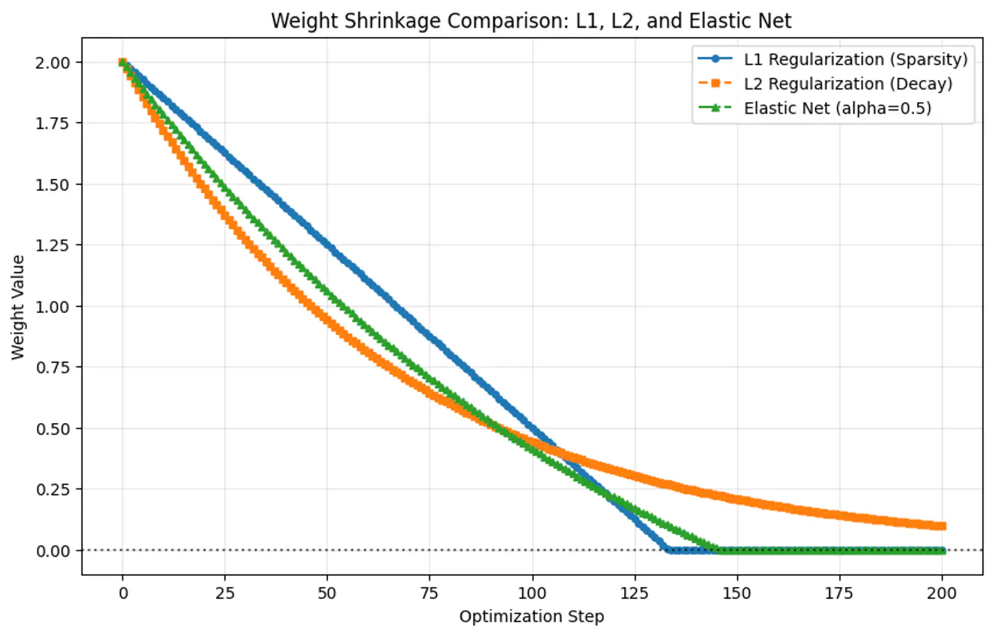
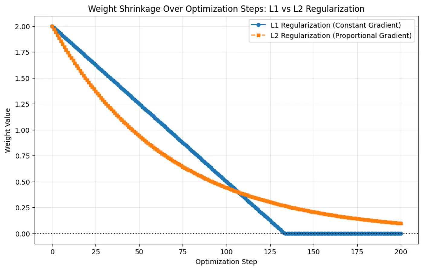
- Because the gradient of L1 penalty (absolute function) is a constant value, i.e, \(\pm 1\), this means a constant reduction in weight at each step, making it gradually reach to 0 in finite steps.
- Whereas, the derivative of L2 penalty is proportional to the weight (\(2w_j\)) and as the weight reaches close to 0, the gradient also becomes very small, this means that the weight will become very close to 0, but not exactly equal to 0.
End of Section
12 - Regression Metrics
MAE = \(\frac{1}{n} \sum_{i=1}^n |y_i - \hat{y_i}|\)
- Treats each error equally.
- Robust to outliers.
- Not differentiable x=0.
- Using gradient descent requires computational hack.
- Easy to interpret, as same units as target variable.
MSE = \(\frac{1}{n} \sum_{i=1}^n (y_i - \hat{y_i})^2\)
- Heavily penalizes large errors.
- Sensitive to outliers.
- Differentiable everywhere.
- Used by gradient descent and most other optimization algorithms.
- Difficult to interpret, as it has squared units.
RMSE = \(\sqrt{\frac{1}{n} \sum_{i=1}^n (y_i - \hat{y_i})^2}\)
- Easy to interpret, as it has same units as target variable.
- Useful when we need outlier-sensitivity of MSE but the interpretability of MAE.
Measures improvement over mean model.
\[ R^2 = 1 - \frac{SS_{res}}{SS_{tot}} = 1 - \frac{\sum_{i=1}^n (y_i - \hat{y_i})^2}{\sum_{i=1}^n (y_i - \bar{y_i})^2} \]Good R^2 value depends upon the use case, e.g. :
- Car 🚗 sale, R =0.8 is good enough.
- Cancer 🧪 prediction R 0.95, as life depends on it.
Range of values:
- Best value = 1
- Baseline value = 0
- Worst value = \(- \infty\)
Note: Example for bad model is all the points lie along x-axis and model predicts y-axis.
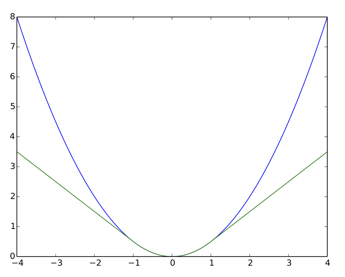
Quadratic for small errors; Linear for large errors.
\[ L_{\delta}(y, \hat{y}) = \begin{cases} \frac{1}{2}(y - \hat{y})^2 & \text{for } |y - \hat{y}| \le \delta \\ \\ \delta (|y - \hat{y}| - \frac{1}{2}\delta) & \text{otherwise} \end{cases} \]- Robust to outliers.
- Differentiable at 0; smooth convergence to minima.
- Delta (\(\delta\)) knob(hyper parameter) to control.
- \(\delta\) high: MSE
- \(\delta\) low: MAE
Note: Tune \(\delta\): MAE, for outliers > \(\delta\); MSE, for small errors < \(\delta\).
e.g: = 95th percentile of errors or 1.35\(\sigma\) for standard Gaussian data.
Huber loss (Green) and Squared loss (blue)
End of Section
13 - Assumptions
Linear Regression works reliably only when certain key 🔑 assumptions about the data are met.
- Linearity
- Independence of Errors (No Auto-Correlation)
- Homoscedasticity (Equal Variance)
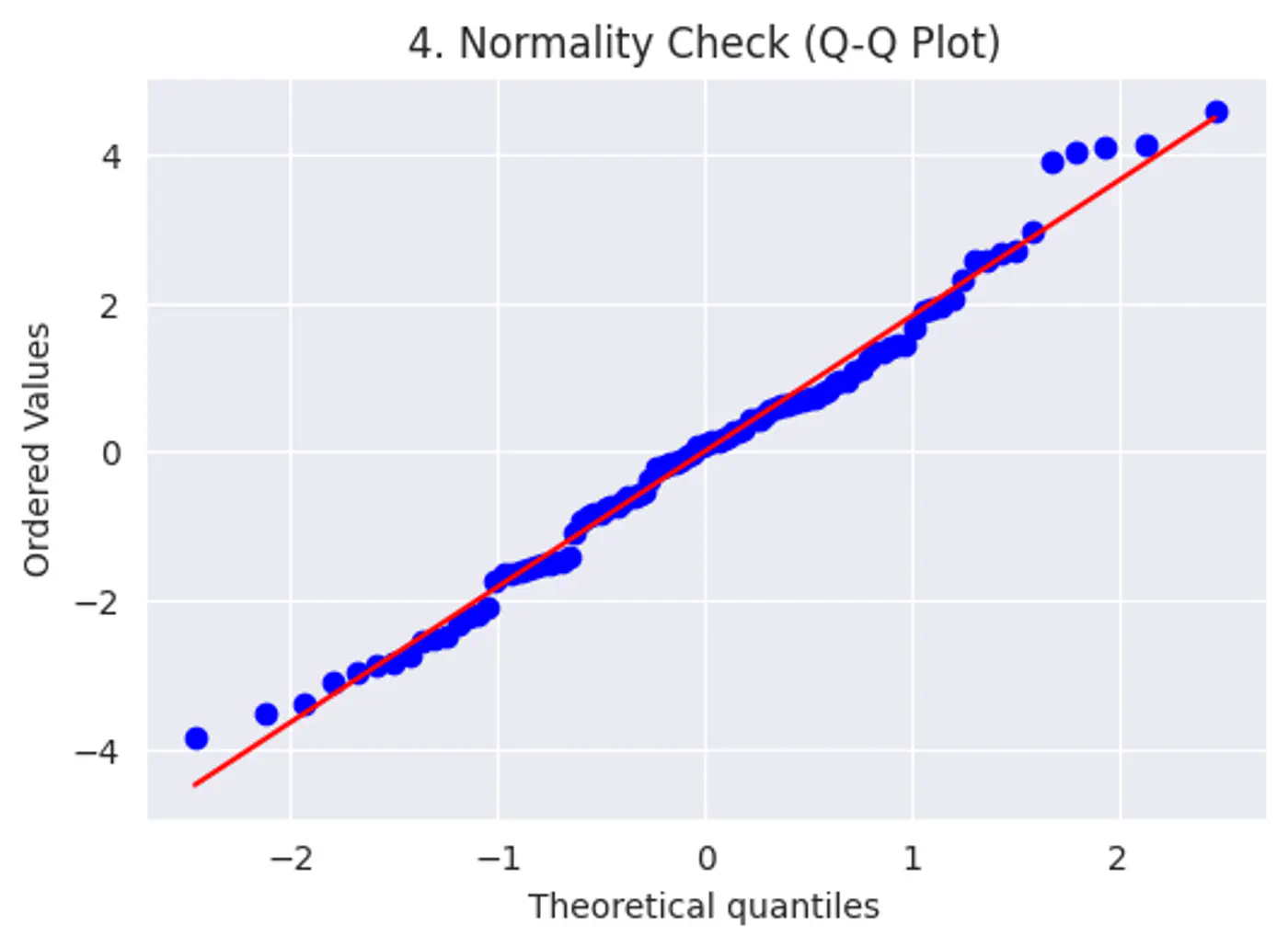
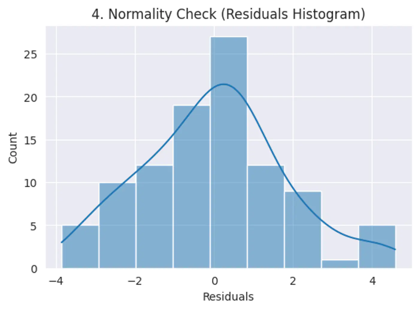
- Normality of Errors
- No Multicollinearity
- No Endogeneity (Target not correlated with the error term)
Relationship between features and target 🎯 is linear in parameters.
Note: Polynomial regression is linear regression.
\(y=w_0 +w_1x_1+w_2x_2^2 + w_3x_3^3\)
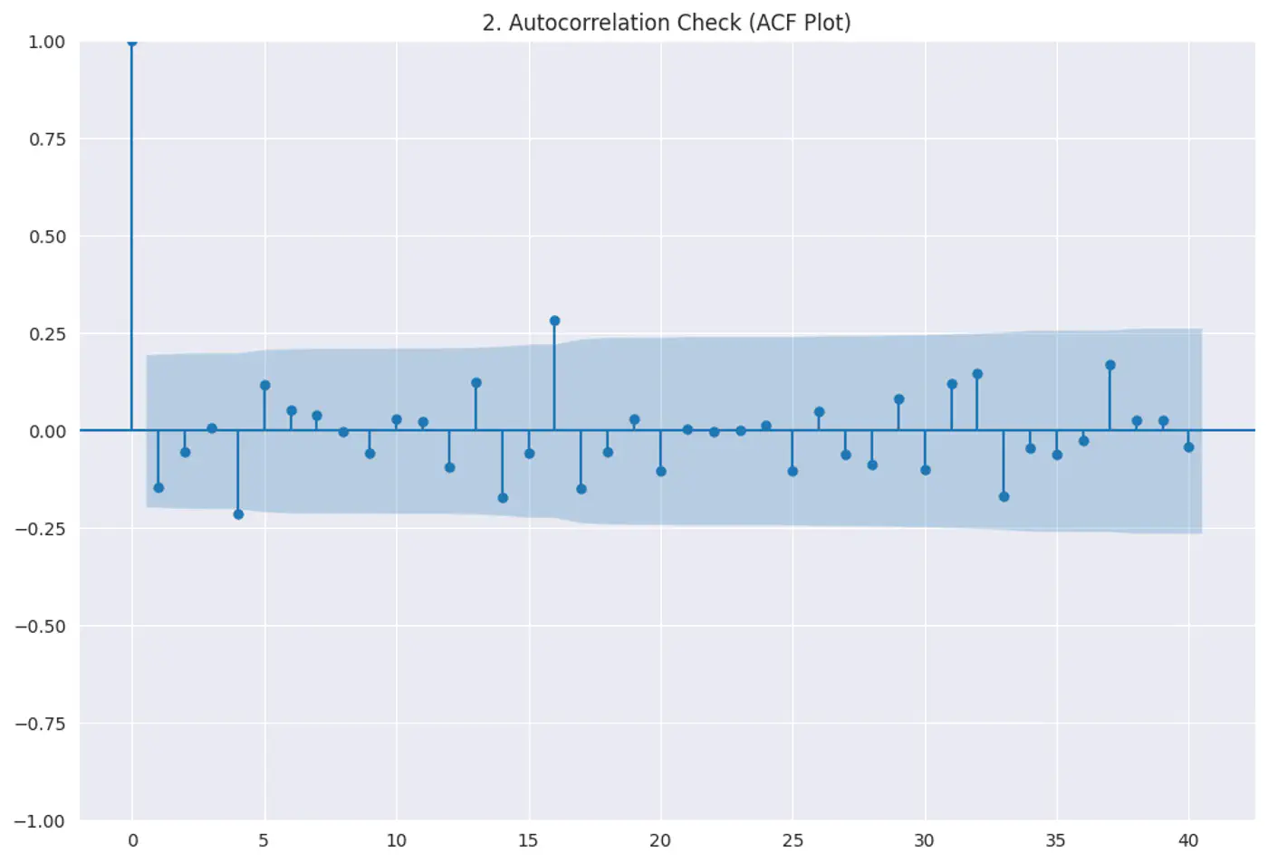
Residuals (errors) should not have a visible pattern or correlation with one another (most common in time-series ⏰ data).
Risk:
If errors are correlated, standard errors will be underestimated, making variables look ‘statistically significant’ when they are not.
Test:
Durbin–Watson test
Autocorrelation plots (ACF)
Residuals vs time
Constant variance of errors; Var(ϵ|X)=σ
Risk:
Standard errors become biased, leading to unreliable hypothesis tests (t-tests, F-tests).
Test:
- Breusch–Pagan test
- White test
Fix:
- Log transform
- Weighted Least Squares(WLS)
Error terms should follow a normal distribution; (Required for small datasets.)
Note: Because of Central Limit Theorem, with a large enough sample size, this becomes less critical for estimation.
Risk: Hypothesis testing (calculating p-values and confidence intervals), we assume the error terms follow a normal distribution.
Test:
Q-Q plot
Shapiro-Wilk Test
Features should not be highly correlated with each other.
Risk:
- High correlation makes it difficult to determine the unique, individual impact of each feature. This leads to high variance in model parameter estimates, small changes in data cause large swings in parameters.
- Model interpretability issues.
Test:
- Variance Inflation Factor(VIF)VIF > 5 → concern, VIF > 10 → serious issue
Fix:
- PCA
- Remove redundant features
Error term must be uncorrelated with the features; E[ϵ|X] = 0
Risk:
- Parameters will be biased and inconsistent.
Test:
- Hausman Test
- Durbin-Wu-Hausman (DWH) Test
Fix:
- Controlled experiments.
End of Section