This is the multi-page printable view of this section. Click here to print.
Logistic Regression
1 - Binary Classification
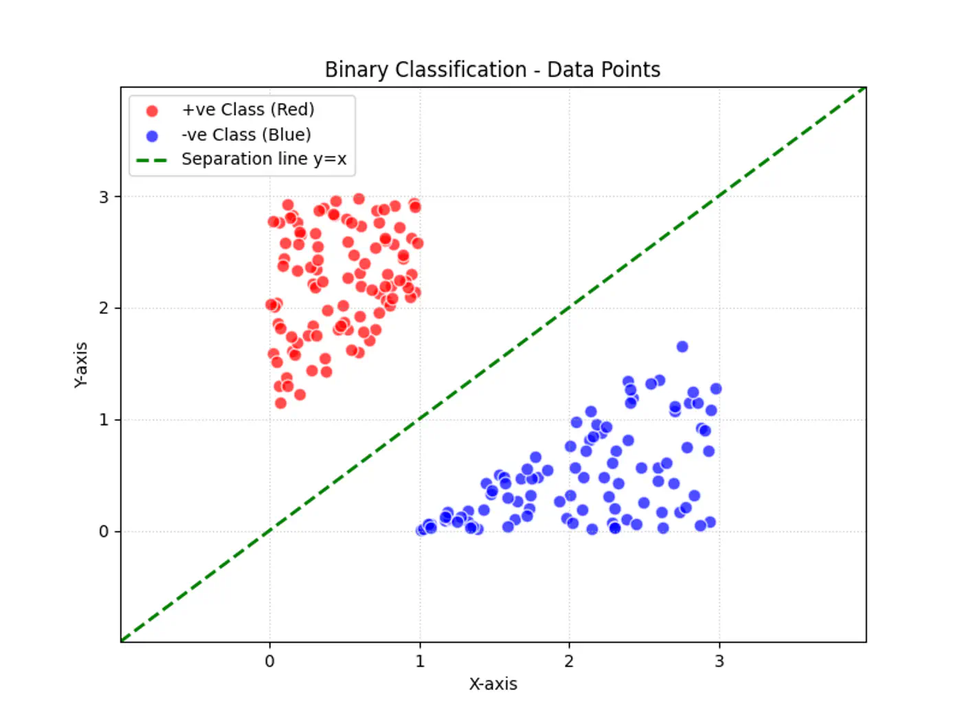
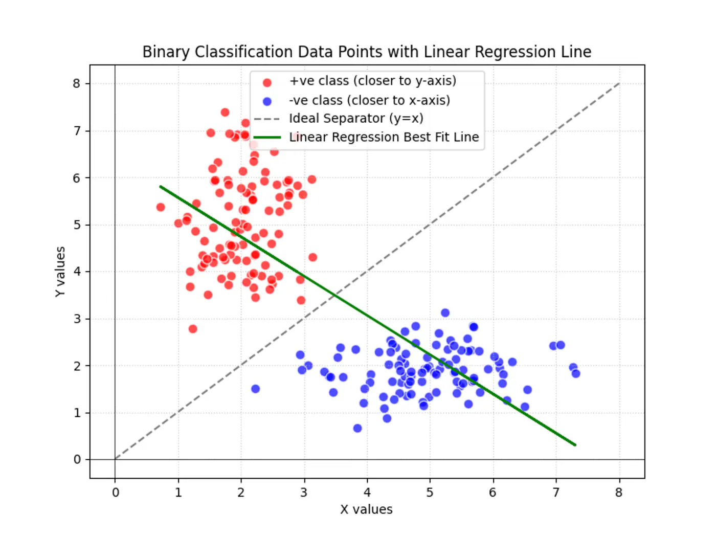
Linear regression tries to find the best fit line, but we want to find the line or decision boundary that clearly separates the two classes.
Find the decision boundary, i.e, the equation of the separating hyperplane.
\[z=w^{T}x+w_{0}\]Value of \(z = \mathbf{w^Tx} + w_0\) tells us how far is the point from the decision boundary and on which side.
Note: Weight 🏋️♀️ vector ‘w’ is normal/perpendicular to the hyperplane, pointing towards the positive class (y=1).
- For points exactly on the decision boundary \[z = \mathbf{w^Tx} + w_0 = 0 \]
- Positive (+ve) labeled points \[ z = \mathbf{w^Tx} + w_0 > 0 \]
- Negative (-ve) labeled points \[ z = \mathbf{w^Tx} + w_0 < 0 \]
So we need a link 🔗 to transform the geometric distance to probability.
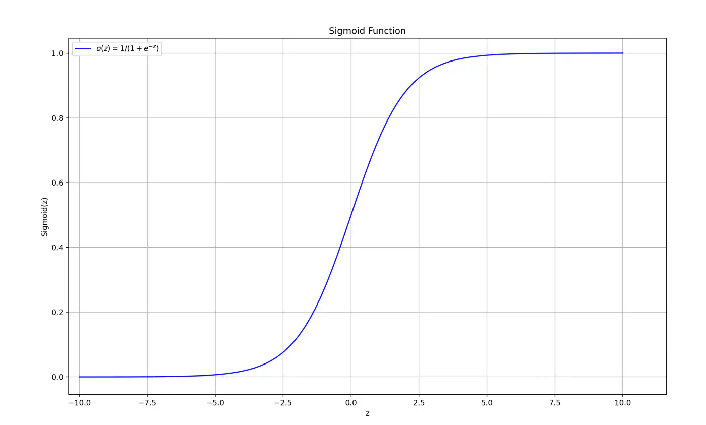
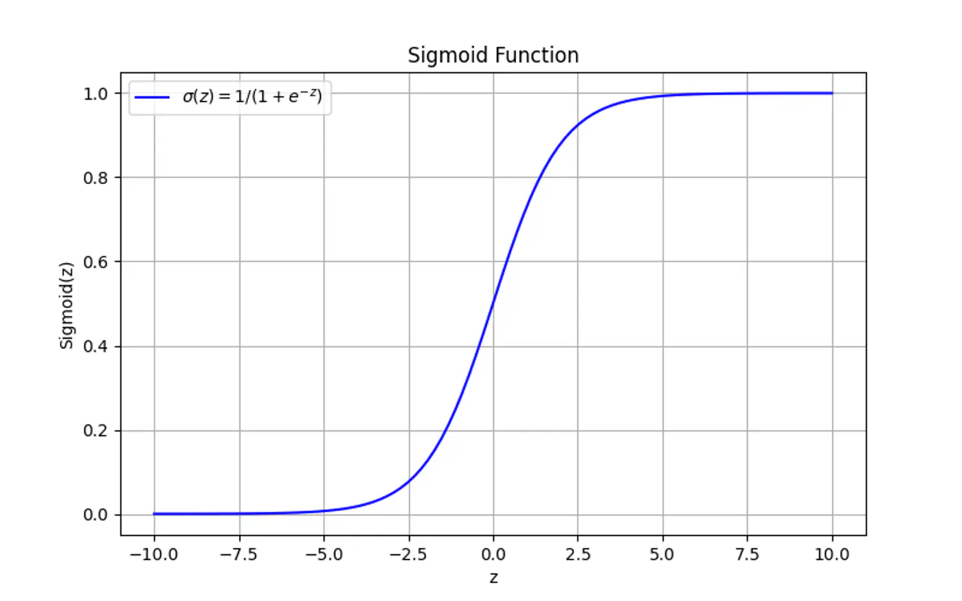
Maps the output of a linear equation to a value between 0 and 1, allowing the result to be interpreted as a probability.
\[\hat{y} = \sigma(z) = \frac{1}{1 + e^{-z}}\]If the distance ‘z’ is large and positive, \(\hat{y} \approx 1\) (High confidence).
If the distance ‘z’ is 0, \(\hat{y} = 0.5\) (Maximum uncertainty).
End of Section
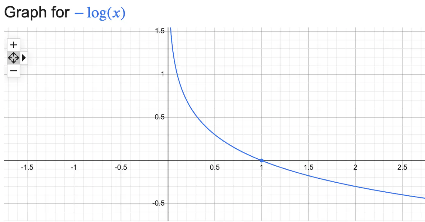
2 - Log Loss
Log Loss = \(\begin{cases} -log(\hat{y_i}) & \text{if } y_i = 1 \\ \\ -log(1-\hat{y_i}) & \text{if } y_i = 0 \end{cases} \)
Combining the above 2 conditions into 1 equation gives:
Log Loss = \(-[y_ilog(\hat{y_i}) + (1-y_i)log(1-\hat{y_i})]\)
We need to find the weights 🏋️♀️ ‘w’ that minimize the cost 💵 function.
- Weight update: \[w_{new}=w_{old}-η.\frac{∂J(w)}{∂w_{old}}\]
We need to find the gradient of log loss w.r.t weight ‘w’.
Chain Rule:
\[\frac{\partial{J(w)}}{\partial{w}} = \frac{\partial{J(w)}}{\partial{\hat{y}}}.\frac{\partial{\hat{y}}}{\partial{z}}.\frac{\partial{z}}{\partial{w}}\]- Cost Function: \(J(w) = -\frac{1}{n}\sum [y_ilog(\hat{y_i}) + (1-y_i)log(1-\hat{y_i})]\)
- Prediction: \(\hat{y} = \sigma(z) = \frac{1}{1 + e^{-z}}\)
- Distance of Point: \(z = \mathbf{w^Tx} + w_0\)
How loss changes w.r.t prediction ?
\[ \begin{align*} \frac{\partial{J(w)}}{\partial{\hat{y}}} &= - [\frac{y}{\hat{y}} - \frac{1-y}{1-\hat{y}}] \\ &= -[\frac{y- \cancel{y\hat{y}} -\hat{y} + \cancel{y\hat{y}}}{\hat{y}(1-\hat{y})}] \\ \therefore \frac{\partial{J(w)}}{\partial{\hat{y}}} &= \frac{\hat{y} - y}{\hat{y}(1-\hat{y})} \end{align*} \]How prediction changes w.r.t distance ?
\[ \begin{align*} \frac{\partial{\hat{y}}}{\partial{z}} &= \frac{\partial{\sigma(z)}}{\partial{z}} = \sigma'(z) \\ \sigma'(z) &= \sigma(z)(1-\sigma(z)) \\ \therefore \frac{\partial{\hat{y}}}{\partial{z}} &= \hat{y}(1-\hat{y}) \end{align*} \]from equations (1) & (2):
\[ \begin{align*} \because \frac{\partial{\sigma(z)}}{\partial{z}} &= \frac{\partial{\sigma(z)}}{\partial{u}}. \frac{\partial{u}}{\partial{z}} \\ \implies \frac{\partial{\sigma(z)}}{\partial{z}} &= - \frac{1}{(1 + e^{-z})^2}. -e^{-z} = \frac{e^{-z}}{(1 + e^{-z})^2} \\ 1 - \sigma(z) & = 1 - \frac{1}{1 + e^{-z}} = \frac{e^{-z}}{1 + e^{-z}} \\ \frac{\partial{\sigma(z)}}{\partial{z}} &= \frac{1}{1 + e^{-z}}.\frac{e^{-z}}{1 + e^{-z}} \\ \therefore \frac{\partial{\sigma(z)}}{\partial{z}} &= \sigma(z).(1-\sigma(z)) \end{align*} \]How distance changes w.r.t weight 🏋️♀️ ?
\[ \frac{\partial{z}}{\partial{w}} = \mathbf{x} \]\[\because \frac{\partial{(a^T\mathbf{x})}}{\partial{\mathbf{x}}} = a\]Chain Rule:
\[ \begin{align*} \frac{\partial{J(w)}}{\partial{w}} &= \frac{\partial{J(w)}}{\partial{\hat{y}}}.\frac{\partial{\hat{y}}}{\partial{z}}.\frac{\partial{z}}{\partial{w}} \\ &= \frac{\hat{y} - y}{\cancel{\hat{y}(1-\hat{y})}}.\cancel{\hat{y}(1-\hat{y})}.x \\ \therefore \frac{\partial{J(w)}}{\partial{w}} &= (\hat{y} - y).x \end{align*} \]Gradient = Error x Input
- Error = \((\hat{y_i}-y_i)\): how far is prediction from the truth?
- Input = \(x_i\): contribution of specific feature to the error.
Weight update:
\[w_{new} = w_{old} - \eta. \sum_{i=1}^n (\hat{y_i} - y_i).x_i\]Mean Squared Error (MSE) can not be used to quantify error/loss in binary classification because:
- Convexity : MSE combined with Sigmoid is non-convex, so, Gradient Descent can get trapped in local minima.
- Penalty: MSE does not appropriately penalize mis-classifications in binary classification.
- e.g: If actual value is class 1 but the model predicts class 0, then MSE = \((1-0)^2 = 1\), which is very low, whereas log loss = \(-log(0) = \infty\)
End of Section
3 - Regularization
The weights 🏋️♀️ will tend towards infinity, preventing a stable solution.
The model tries to make probabilities exactly 0 or 1, but the sigmoid function never reaches these limits, leading to extreme weights 🏋️♀️ to push probabilities near the extremes.
Distance of Point: \(z = \mathbf{w^Tx} + w_0\)
Prediction: \(\hat{y} = \sigma(z) = \frac{1}{1 + e^{-z}}\)
Log loss: \(-[y_ilog(\hat{y_i}) + (1-y_i)log(1-\hat{y_i})] \)
Model becomes perfectly accurate on training 🏃♂️data but fails to generalize, performing poorly on unseen data.
Adds a penalty term to the loss function, discouraging weights 🏋️♀️ from becoming too large.
End of Section
4 - Log Odds
Odds compare the likelihood of an event happening vs. not happening.
Odds = \(\frac{p}{1-p}\)
- p = probability of success
In logistic regression we assume that Log-Odds (the log of the ratio of positive class to negative class) is a linear function of inputs.
Log-Odds (Logit) = \(log_e \frac{p}{1-p}\)
Log Odds = \(log_e \frac{p}{1-p} = z\)
\[z=w^{T}x+w_{0}\]\[ \begin{align*} &log_{e}(\frac{p}{1-p}) = z \\ &⟹\frac{p}{1-p} = e^{z} \\ &\implies p = e^z - p.e^z \\ &\implies p = \frac{e^z}{1+e^z} \\ &\text { divide numerator and denominator by } e^z \\ &\implies p = \frac{1}{1+e^{-z}} \quad \text { i.e, Sigmoid function} \end{align*} \]- Probability: 0 to 1
- Odds: 0 to + \(\infty\)
- Log Odds: -\(\infty\) to +\(\infty\)
End of Section
5 - Probabilistic Interpretation
We assume that our target variable ‘y’ follows a Bernoulli distribution, i.e, has exactly 2 outputs success/failure.
- P(Y=1|X) = p
- P(Y=0|X) = 1- p
Combining above 2 into 1 equation gives:
- P(Y=y|X) = \(p^y(1-p)^{1-y}\)
‘Find the most plausible explanation for what I see.’
We want to find the weights 🏋️♀️‘w’ that maximize the likelihood of seeing the data.
- Data, D = \(\{ (x_i, y_i)_{i=1}^n , \quad y_i \in \{0,1\} \}\)
We do this by maximizing likelihood function.
Assumption: Training data is I.I.D.
A common simplification is to maximize the log-likelihood function instead, which converts the product into a sum.
Note: Log is a strictly monotonically increasing function.
Maximizing the log-likelihood is same as minimizing the negative of log-likelihood.
\[ \begin{align*} \underset{w}{\mathrm{max}}\ log\mathcal{L}(w) &= \underset{w}{\mathrm{min}} - log\mathcal{L}(w) \\ \underset{w}{\mathrm{min}} - log\mathcal{L}(w) &= - \sum_{i=1}^n [ y_ilog(p_i) + (1-y_i)log(1-p_i)] \\ \underset{w}{\mathrm{min}} - log\mathcal{L}(w) &= \text {Log Loss} \end{align*} \]End of Section