📌Let’s understand Naive Bayes through an Email/Text classification example.

• Number of words in an email is not fixed.
• Remove all stop words, such as, the, is , are, if, etc.
• Keep only relevant words, i.e, \(w_1, w_2, \dots , w_d\) words.
• We want to do a binary classification - Spam/Not Spam.

Let’s revise Bayes’ theorem first:

• \(P(S|W)\) is the posterior probability: the probability of the email being spam, given the words inside it.
• \(P(W|S)\) is the likelihood: how likely is this email’s word pattern if it were spam?
• \(P(S)\) is the prior probability: The ‘base rate’ of spam.
  • If our dataset has 10,000 emails and 2,000 are spam, then \(P(S)\)=0.2.
• \(P(W)\) is the prior probability of the predictor (evidence): total probability of seeing these words across all emails.
  • 👉Since this is the same for both classes, we treat it as a constant and ignore it during comparison.

👉Likelihood = \(P(W|S)\) = \(P(w_1, w_2, \dots w_d | S)\)

➡️ For computing the joint distribution of say d=1000 words, we need to learn from possible \(2^{1000}\) combinations.

• \(2^{1000}\) > the atoms in the observable 🔭 universe 🌌.
• We will never have enough training data to see every possible combination of words even once.
  • Most combinations would have a count of zero.

🦉So, how do we solve this ?

💡The ‘Naive’ assumption is a ‘Conditional Independence’ assumption, i.e, we assume each word appears independently of the others, given the class Spam/Not Spam.

• e.g. In a spam email, the likelihood of ‘Free’ and ‘Money’ 💵 appearing are treated as independent events, even though they usually appear together.

Note: The conditional independence assumption makes the probability calculations easier, i.e, the joint probability simply becomes the product of individual probabilities, conditional on the label.

We can generalize it for any number of class labels ‘y’:

Note: We compute the probabilities for both Spam/Not Spam and assign the final label to email, depending upon which probability is higher.

👉Space Complexity: O(d*c)

👉Time Complexity:

• Training: O(n*d*c)
• Inference: O(d*c)

Where,

• d = number of features/dimensions
• c = number of classes
• n = number of training examples

⭐️Simple, fast, and highly effective probabilistic machine learning classifier based on Bayes’ theorem.

🦀What if at runtime we encounter a word that was never seen during training ?

e.g. A word ‘crypto’ appears in the test email that was not present in training emails; P(‘crypto’|S) =0.

👉This will force the entire product to zero.

💡Add ‘Laplace smoothing’ to all likelihoods, both during training and test time, so that the probability becomes non-zero.

• \(count(x_{i},y)\) : number of times word appears in documents of class ‘y'.
• \(count(y)\): The total count of all words in documents of class ‘y'.
• \(|V|\)(or \(N_{features}\)):Vocabulary size or total number of unique possible words.

Let’s understand this by the examples below:

1. \(count(w_{i},S) = 0 \), \(count(S) = 100\), \(|V|\)(or \(N_{features}) =2, \alpha = 1\) \[P(w_{i}|S)=\frac{ 0+1 }{100 +1 \cdot 2} = \frac{1}{102}\]
2. \(count(w_{i},S) = 0 \), \(count(S) = 100\), \(|V|\)(or \(N_{features}) =2, \alpha = 10,000\) \[P(w_{i}|S)=\frac{ 0+10,000 }{100 +10,000 \cdot 2} = \frac{10,000}{20,100} \approx \frac{1}{2}\]

Note: High alpha value may lead to under-fitting; \(\alpha = 1\) recommended.

🦀What happens if the number of words ‘d’ is very large ?

👉Multiplying 500 times will result in a number so small a computer 💻 cannot store it (underflow).

Note: Computers have a limit to store floating point numbers, e.g., 32 bit: \(1.175 x 10^{-38}\)

💡Take ‘Logarithm’ that will convert the product to sum.

Note: In the next section we will solve a problem covering all the concepts discussed in this section.

⭐️Simple, fast, and highly effective probabilistic machine learning classifier based on Bayes’ theorem.

Let’s solve an email classification problem, below we have list of emails (tokenized) and labelled as Spam/Not Spam for training.

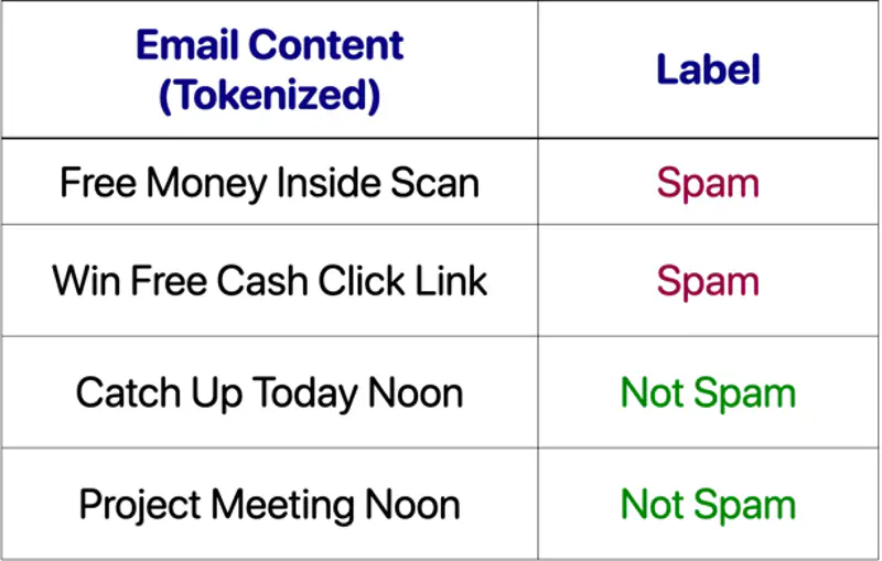
🏛️Class Priors:

• P(Spam) = 2/4 =0.5
• P(Not Spam) = 2/4 = 0.5

📕 Vocabulary = { Free, Money, Inside, Scan, Win, Cash, Click, Link, Catch, Up Today, Noon, Project, Meeting }

• |V| = Total unique word count = 14

🧮 Class count:

• count(Spam) = 9
• count(Not Spam) = 7

✅ Laplace smoothing: \(\alpha = 1\)

• P(‘free’| Spam) = \(\frac{2+1}{9+14} = \frac{3}{23} = 0.13\)
• P(‘free’| Not Spam) = \(\frac{0+1}{7+14} = \frac{1}{21} = 0.047\)

👉Say a new email 📧 arrives - “Free money today”; lets classify it as Spam/Not Spam.

Spam:

• P(‘free’| Spam) = \(\frac{2+1}{9+14} = \frac{3}{23} = 0.13\)
• P(‘money’| Spam) = \(\frac{1+1}{9+14} = \frac{2}{23} = 0.087\)
• P(‘today’| Spam) = \(\frac{0+1}{9+14} = \frac{1}{23} = 0.043\)

Not Spam:

• P(‘free’| Not Spam) = \(\frac{0+1}{7+14} = \frac{1}{21} = 0.047\)
• P(‘money’| Not Spam) = \(\frac{0+1}{7+14} = \frac{1}{21} = 0.047\)
• P(‘today’| Not Spam) = \(\frac{1+1}{7+14} = \frac{2}{21} = 0.095\)

• Score(Spam) = log(P(Spam)) + log(P(‘free’|S)) + log(P(‘money’|S)) + log(P(‘today’|S))
  = log(0.5) + log(0.13) + log(0.087) + log(0.043) = -0.301 -0.886 -1.06 -1.366 = -3.614
• Score(Not Spam) = log(P(Not Spam)) + log(P(‘free’|NS)) + log(P(‘money’|NS)) + log(P(‘today’|NS))
  = log(0.5) + log(0.047) + log(0.047) + log(0.095) = -0.301 -1.328 -1.328 -1.022 = -3.979

👉Since, Score(Spam) (-3.614 )> Score(Not Spam) (-3.979) , the model chooses ‘Spam’ as the label for the email.