This is the multi-page printable view of this section. Click here to print.
Support Vector Machine
1 - SVM Intro
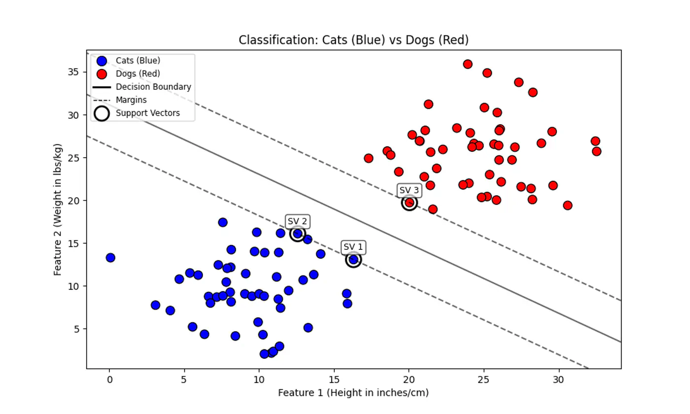
⭐️We have two classes of points (e.g. Cats 😸vs. Dogs 🐶) that can be separated by a straight line.
👉 Many such lines exist !
💡SVM asks: “Which line is the safest?”
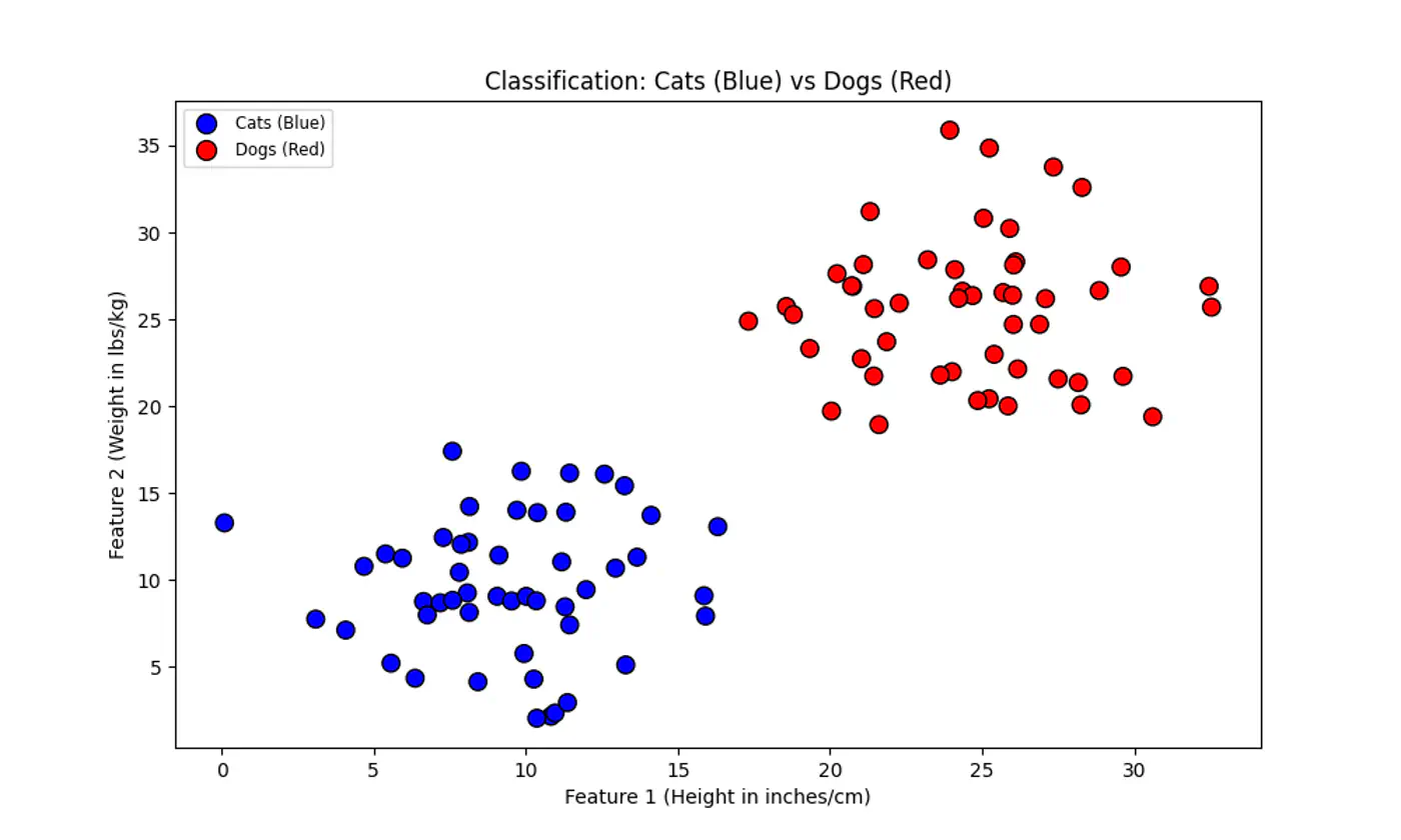
💡Think of the decision boundary as the center-line of a highway 🛣️.
SVM tries to make this highway 🛣️ as wide as possible without hitting any ‘buildings’ 🏡 (data points) on either side.
End of Section
2 - Hard Margin SVM
Data is perfectly linearly separable, i.e, there must exist a hyperplane that can perfectly separate the data into two distinct classes without any misclassification.
No noise or outliers that fall within the margin or on the wrong side of the decision boundary. Note: Even a single outlier can prevent the algorithm from finding a valid solution or drastically affect the boundary’s position, leading to poor generalization.
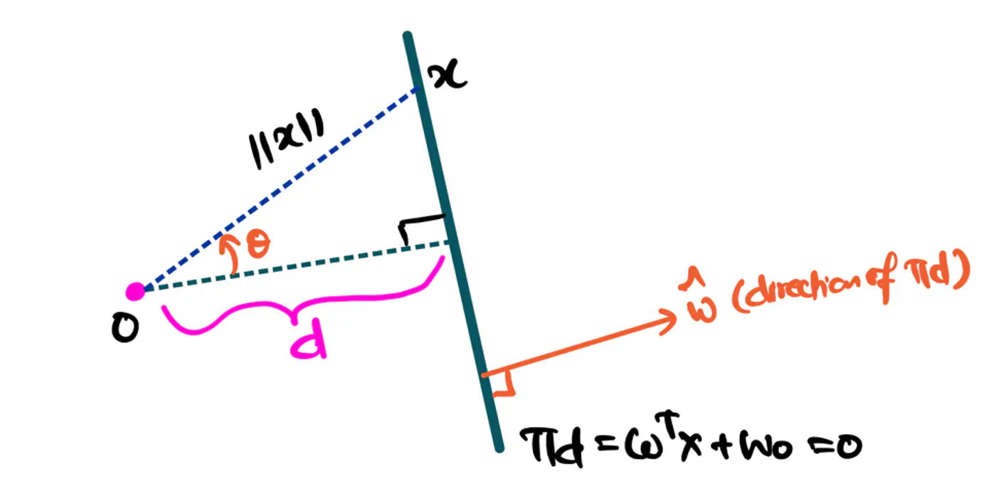
- 🐎 Distance(signed) of a hyperplane from origin = \(\frac{-w_0}{\|w\|}\)
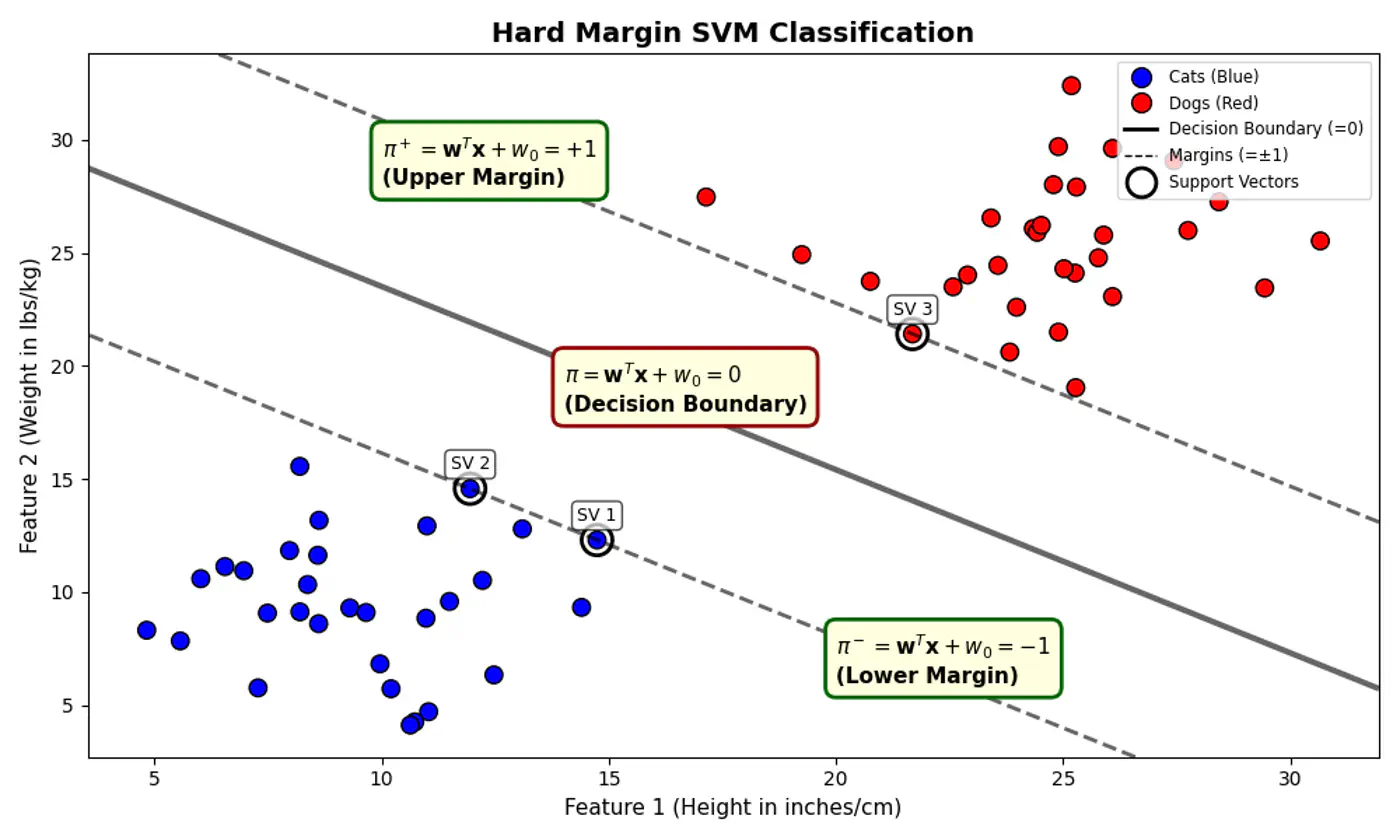
- 🦣 Margin width = distance(\(\pi^+, \pi^-\))
- = \(\frac{1-w_0 - (-1 -w_0)}{\|w\|}\) = \(\frac{1-\cancel{w_0} + 1 + \cancel{w_0})}{\|w\|}\)
- distance(\(\pi^+, \pi^-\)) = \(\frac{2}{\|w\|}\)
Figure: Distance of Hyperplane from Origin
- Separating hyperplane \(\pi\) is exactly equidistant from \(\pi^+\) and \(\pi^-\).
- We want to maximize the margin between +ve(🐶) and -ve (😸) points.
👉Combining above two constraints:
\[y_{i}.(w^{T}x_{i}+w_{0})≥1\]such that, \(y_i.(w^Tx_i + w_0) \ge 1\)
👉To maximize the margin, we must minimize \(\|w\|\).
Since, distance(\(\pi^+, \pi^-\)) = \(\frac{2}{\|w\|}\)
such that, \(y_i.(w^Tx_i + w_0) \ge 1 ~ \forall i = 1,2,\dots, n\)
Note: Hard margin SVM will not work if the data has a single outlier or slight overlap.
End of Section
3 - Soft Margin SVM
💡Imagine the margin is a fence 🌉.
Hard Margin: fence is made of steel.
Nothing can cross it.Soft Margin: fence is made of rubber(porous).
Some points can ‘push’ into the margin or even cross over to the wrong side, but we charge them a penalty 💵 for doing so.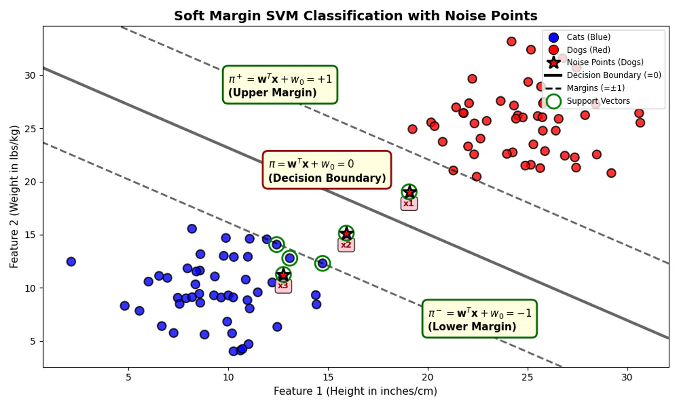
Distance from decision boundary:
- Distance of positive labelled points must be \(\ge 1\)
- But, distance of noise 📢 points (actually positive points) \(x_1, x_2 ~\&~ x_3\) < 1
⚔️ So, we introduce a slack variable or allowance for error term, \(\xi_i\) (pronounced ‘xi’) for every single data point.
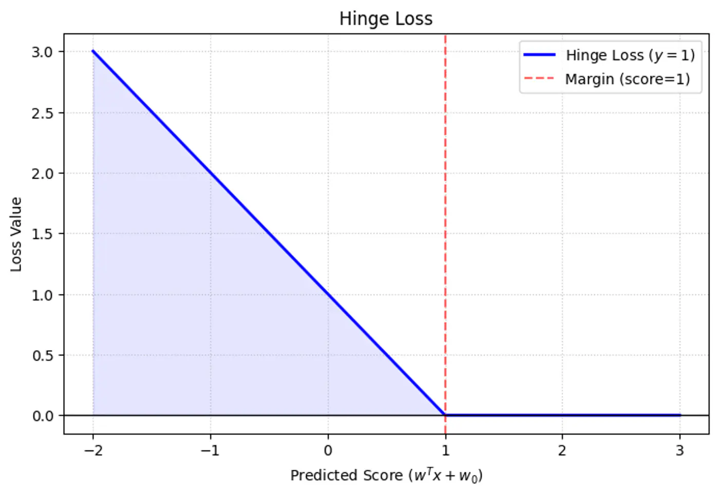
\[y_i.(w^Tx_i + w_0) \ge 1 - \xi_i, ~ \forall i = 1,2,\dots, n\]\[ \implies \xi_i \ge 1 - y_i.(w^Tx_i + w_0) \\ also, ~ \xi_i \ge 0 \]\[So, ~ \xi _{i}=\max (0,1-y_{i}\cdot (w^Tx_i + w_0))\]Note: The above error term is also called ‘Hinge Loss’.
Hinge
- \(\xi_i = 0\) : Correctly classified and outside (or on) the margin.
- \(0 < \xi_i \le 1 \) : Within the margin but on the correct side of the decision boundary.
- \(\xi_i > 0\): On the wrong side of the decision boundary (misclassified).
e.g.: Since, the noise 📢 point are +ve (\(y_i=1\)) labeled:
\[\xi _{i}=\max (0,1-f(x_{i}))\]\(x_1, (d=+0.5)\): \(\xi _{i}=\max (0,1-0.5) = 0.5\)
\(x_2, (d=-0.5)\): \(\xi _{i}=\max (0,1-(-0.5))= 1.5\)
\(x_3, (d=-1.5)\): \(\xi _{i}=\max (0,1-(-1.5)) = 2.5\)

Subject to constraints:
- \(y_i(w^T x_i + b) \geq 1 - \xi_i\): The ‘softened’ margin constraint.
- \(\xi_i \geq 0\): Slack/Error cannot be negative.
Note: We use a hyper-parameter ‘C’ to control the trade-off.
- Large ‘C’: Over-Fitting;
Misclassifications are expensive 💰.
Model tries to keep the errors as low as possible. - Small ‘C’: Under-Fitting;
Margin width is more important than individual errors.
Model will ignore outliers/noise to get a ‘cleaner’(wider) boundary.
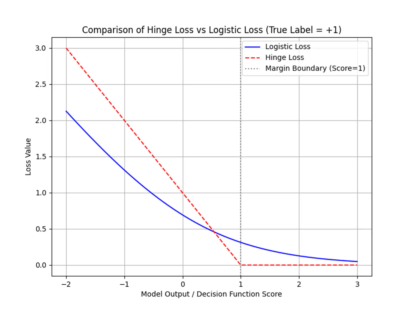
Note: SVM is just L2-Regularized Hinge Loss minimization, as Logistic Regression minimizes Log-Loss.
End of Section
4 - Primal Dual Equivalence
The Primal form is intuitive but computationally expensive in high dimensions.
➡️ Number of new features = \({d+p \choose p}\), grows roughly as \(O(d^{p})\)
- d= number of dimensions (features)
- p = degree of polynomial
Note: The Dual form is what enables the Kernel Trick 🪄.
Subject to constraints:
- \(y_i(w^T x_i + b) \geq 1 - \xi_i\): The ‘softened’ margin constraint.
- \(\xi_i \geq 0\): Slack/Error cannot be negative.
⭐️ We start with the Soft-Margin Primal objective and incorporate its constraints using Lagrange Multipliers \((\alpha_i, \mu_i \geq 0)\)
\[L(w, w_0, \xi, \alpha, \mu) = \frac{1}{2}\|w\|^2 + C \sum_{i=1}^n \xi_i - \sum_{i=1}^n \alpha_i \left[y_i(w^T x_i + w_0) - 1 + \xi_i \right] - \sum_{i=1}^n \mu_i \xi_i\]Note: Inequality conditions must be \(\le 0\).
👉The Lagrangian function has two competing objectives:
\[L(w, w_0, \xi, \alpha, \mu) = \frac{1}{2}\|w\|^2 + C \sum_{i=1}^n \xi_i - \sum_{i=1}^n \alpha_i \left[y_i(w^T x_i + w_0) - 1 + \xi_i \right] - \sum_{i=1}^n \mu_i \xi_i\]- Minimization: We want to minimize \(L(w, w_0, \xi, \alpha, \mu)\) w.r.t primal variables (\(w, w_0, \xi_i \) ) to find the hyperplane with the largest possible margin.
- Maximization: We want to maximize \(L(w, w_0, \xi, \alpha, \mu)\) w.r.t dual variables (\(\alpha_i, \mu_i\) ) to ensure all training constraints are satisfied.
Note: A point that is simultaneously a minimum for one set of variables and a maximum for another is, by definition, a saddle point.
👉To find the Dual, we find the saddle point by taking partial derivatives with respect to the primal variables \((w, w_0, \xi)\) and equating them to 0.
\[\frac{\partial L}{\partial w} = 0 \implies \mathbf{w = \sum_{i=1}^n \alpha_i y_i x_i}\]\[\frac{\partial L}{\partial w_0} = 0 \implies \mathbf{\sum_{i=1}^n \alpha_i y_i = 0}\]\[\frac{\partial L}{\partial \xi_i} = 0 \implies C - \alpha_i - \mu_i = 0 \implies \mathbf{0 \leq \alpha_i \leq C}\]subject to: \(0 \leq \alpha_i \leq C\) and \(\sum \alpha_i y_i = 0\)
- \(\alpha_i\)= 0, for non support vectors (correct side)
- \(0 < \alpha_i < C\), for free support vectors (exactly on the margin)
- \(\alpha_i = C\), for bounded support vectors (misclassified or inside margin)
Note: Sequential Minimal Optimization (SMO) algorithm is used to find optimal \(\alpha_i\) values.
🎯To classify unseen point \(x_q\) : \(f(x_q) = \text{sign}(w^T x_q + w_0)\)
✅ From the KKT stationarity condition, we know: \(\mathbf{w} = \sum_{i=1}^n \alpha_i y_i x_i\)
👉 Substituting this into the equation:
\[f(x_q) = \text{sign}\left( \sum_{i=1}^n \alpha_i y_i (x_i^T x_q) + w_0 \right)\]Note: Even if you have 1 million training points, if only 500 are support vectors, the summation only runs for 500 terms.
All other points have \(\alpha_i = 0\) and vanish.
End of Section
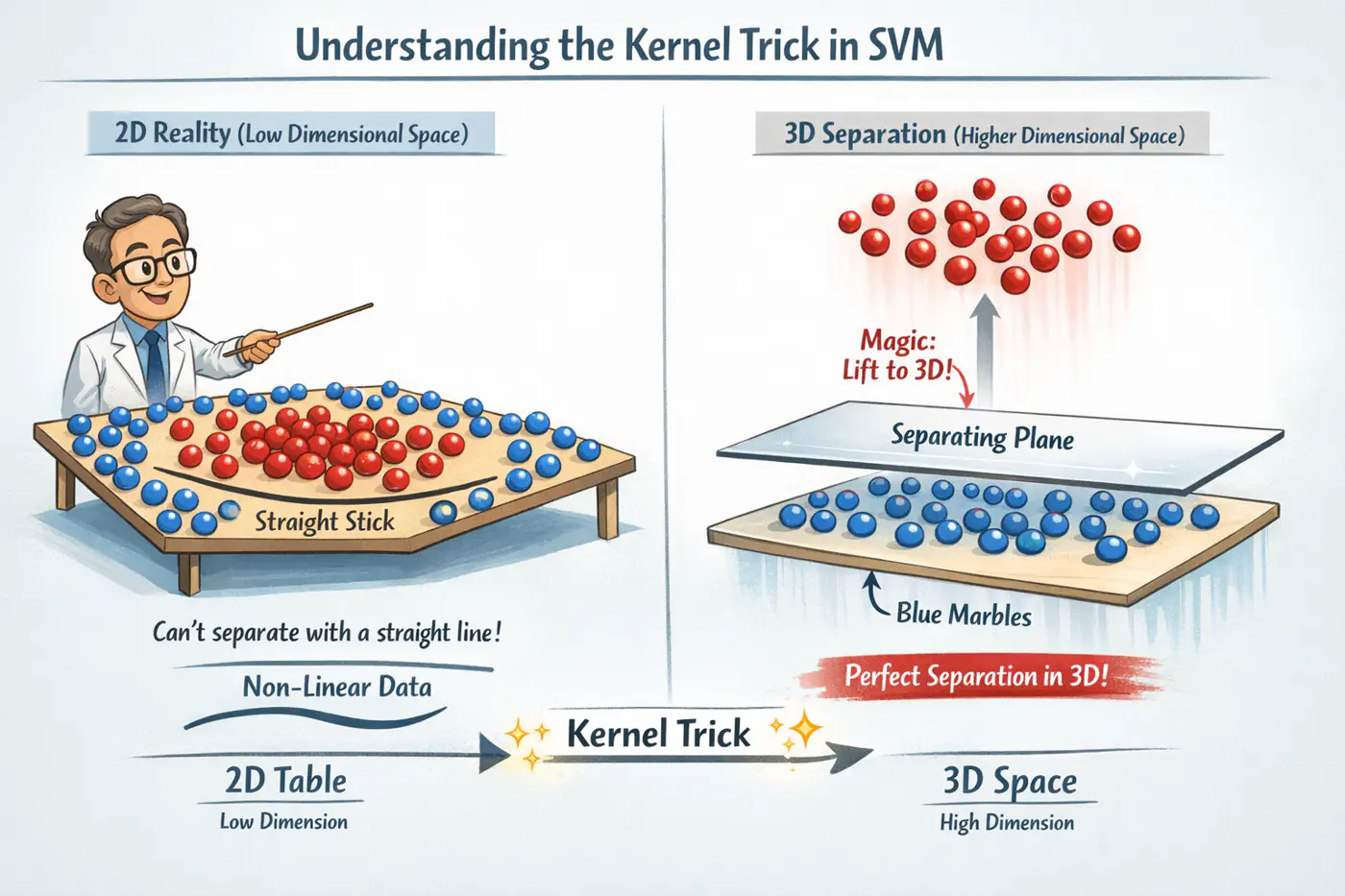
5 - Kernel Trick
👉If our data is not linearly separable in its original space , we can map it to a higher-dimensional feature space (where D»d) using a transformation function .
- Bridge between Dual formulation and the geometry of high dimensional spaces.
- It is a way to manipulate inner product spaces without the computational cost 💰 of explicit transformation.
subject to: \(0 \leq \alpha_i \leq C\) and \(\sum \alpha_i y_i = 0\)
💡Actual values of the input vectors \(x_i\) and \(x_j\) never appear in isolation; only appear as inner product.
\[ \max_{\alpha} \sum_{i=1}^n \alpha_i - \frac{1}{2} \sum_{i,j=1}^n \alpha_i \alpha_j y_i y_j \mathbf{(x_i \cdot x_j)}\]\[f(x_q) = \text{sign}\left( \sum_{i=1}^n \alpha_i y_i (x_i^T x_q) + w_0 \right)\]👉The ‘shape’ of the decision boundary is entirely determined by how similar points are to one another, not by their absolute coordinates.
So we define a function called ‘Kernel Function’.
The ‘Kernel Trick’ 🪄 is an optimization that replaces the dot product of a high-dimensional mapping with a function of the dot product in the original space.
\[(x_i, x_j) = \langle \phi(x_i), \phi(x_j) \rangle\]💡How it works ?
Instead of mapping (to higher dimension) \(x_i \rightarrow \phi(x_i)\), \(x_j \rightarrow \phi(x_j)\),
and calculating the dot product.
We simply compute \(K(x_i, x_j)\) directly in the original input space.
👉The ‘Kernel Function’ gives the similar mathematical equivalent of mapping it to a higher dimensions and taking the dot product.
Note: For \(K(x_i, x_j)\) to be a valid kernel, it must satisfy Mercer’s Condition.
Below is an example for a quadratic Kernel function in 2D that is equivalent to mapping the vectors to 3D and taking a dot product in 3D.
\[K(x, z) = (x^T z)^2\]\[(x_1 z_1 + x_2 z_2)^2 = x_1^2 z_1^2 + 2x_1 z_1 x_2 z_2 + x_2^2 z_2^2\]The output of above quadratic kernel function is equivalent to the explicit dot product of two vectors in 3D:
\[\phi(x) = [x_1^2, \sqrt{2}x_1x_2, x_2^2]^T\]\[\phi(z) = [z_1^2, \sqrt{2}z_1z_2, z_2^2]^T\]\[\phi (x)\cdot \phi (z)=x_{1}^{2}z_{1}^{2}+2x_{1}x_{2}z_{1}z_{2}+x_{2}^{2}z_{2}^{2}\]- Computational Efficiency: Avoids the ‘combinatorial blowup’ 💥 of generating thousands of interaction features manually.
- Memory Savings: No need to store 💾 or process high-dimensional coordinates, only the scalar result of the kernel function.
- Designing special purpose domain specific kernel is very hard.
- Basically, we are trying to replace feature engineering with kernel design.
- Note: Deep learning does feature engineering implicitly for us.
- Runtime complexity depends on number of support vectors, whose count is not easy to control.
Note: Runtime Time Complexity ⏰ = \(O(n_{SV}\times d)\) , whereas linear SVM,\(O(d)\) .
End of Section
6 - RBF Kernel
- Unlike the polynomial kernel, which looks at global 🌎 interactions, the RBF kernel acts like a similarity measure.
- If ‘x’ and ‘z’ are identical \(K(x,z)=1\).
- As they move further apart in Euclidean space, the value decays exponentially towards 0.
- If \(x \approx z\) (very close), \(K(x,z)=1\)
- If ‘x’, ‘z’ are far apart, \(K(x,z) \approx 0\)
Note: Kernel function is the measure of similarity or closeness.
Say \(\sigma = 1\), then Euclidean distance: \(\|x - z\|^2 = \|x\|^2 + \|z\|^2 - 2x^Tz\)
\[K(x, z) = \exp(-( \|x\|^2 + \|z\|^2 - 2x^T z )) = \exp(-\|x\|^2) \exp(-\|z\|^2) \exp(2x^T z)\]The Taylor expansion for \(e^u= \sum_{n=0}^{\infty} \frac{u^n}{n!}\)
\[\exp(2x^T z) = \sum_{n=0}^{\infty} \frac{(2x^T z)^n}{n!} = 1 + \frac{2x^T z}{1!} + \frac{(2x^T z)^2}{2!} + \dots + \frac{(2x^T z)^n}{n!} + \dots\]\[K(x, z) = e^{-\|x\|^2} e^{-\|z\|^2} \left( \sum_{n=0}^{\infty} \frac{2^n (x^T z)^n}{n!} \right)\]💡If we expand each \((x^T z)^n\) term, it represents the dot product of all possible n-th order polynomial features.
👉Thus, the implicit feature map is:
\[\phi(x) = e^{-\|x\|^2} \left[ 1, \sqrt{\frac{2}{1!}}x, \sqrt{\frac{2^2}{2!}}(x \otimes x), \dots, \sqrt{\frac{2^n}{n!}}(\underbrace{x \otimes \dots \otimes x}_{n \text{ times}}), \dots \right]^T\]- Important: The tensor product \(x\otimes x\) creates a vector (or matrix) containing all combinations of the features. e.g. if \(x=[x_{1},x_{2}]\), then \(x\otimes x=[x_{1}^{2},x_{1}x_{2},x_{2}x_{1},x_{2}^{2}]\) 
Note: Because the Taylor series has an infinite number of terms, feature map has an infinite number of dimensions.
- High Gamma(low \(\sigma\)): Over-Fitting
- Makes the kernel so ‘peaky’ that each support vector only influences its immediate neighborhood.
- Decision boundary becomes highly irregular, ‘wrapping’ tightly around individual data points to ensure they are classified correctly.
- Low Gamma(high \(\sigma\)): Under-Fitting
- The Gaussian bumps are wide and flat.
- Decision boundary becomes very smooth, essentially behaving more like a linear or low-degree polynomial classifier.
End of Section
7 - Support Vector Regression
👉Imagine a ‘tube’ of radius \(\epsilon\) surrounding the regression line.
- Points inside the tube are considered ‘correct’ and incur zero penalty.
- Points outside the tube are penalized based on their distance from the tube’s boundary.
👉SVR ignores errors as long as they are within a certain distance (\(\epsilon\)) from the true value.
🎯This makes SVR inherently robust to noise and outliers, as it does not try to fit every single point perfectly, only those that ‘matter’ to the structure of the data.
Note: Standard regression (like OLS) tries to minimize the squared error between the prediction and every data point.
Subject to constraints:
- \(y_i - (w^T x_i + w_0) \leq \epsilon + \xi_i\): (Upper boundary)
- \((w^T x_i + w_0) - y_i \leq \epsilon + \xi_i^*\): (Lower boundary)
- \(\xi_i, \xi_i^* \geq 0\): (Slack/Error cannot be negative)
Terms:
- Epsilon(\(\epsilon\)): The width of the tube. Increasing ‘\(\epsilon\)’ results in fewer support vectors and a smoother (flatter) model.
- Slack Variables (\(\xi_i, \xi_i^*\)): How far a point lies outside the upper and lower boundaries of the tube.
- C: The trade-off between the flatness of the model and the extent to which deviations larger than \(\epsilon\) are tolerated.
SVR uses a specific loss function that is 0 when the error<’\(\epsilon\)’.
\[L_\epsilon(y, f(x)) = \max(0, |y - f(x)| - \epsilon)\]- The solution becomes sparse, because the loss is zero for points inside the tube.
- Only the Support Vectors, i.e, points outside or on the boundary of the tube have non-zero Lagrange multipliers (\(\alpha_i\)).
Note: \(\epsilon=0.1\) default value in scikit-learn.
Subject to:
- \(\sum_{i=1}^n (\alpha_i - \alpha_i^*) = 0\)
- \(0 \leq \alpha_i, \alpha_i^* \leq C\)
- \(\alpha_i = \alpha_i^* = 0\): point is inside the tube.
- \(|\alpha_i - \alpha_i^*| > 0\) : support vectors; points on or outside the tube.
Note: \(\alpha_i , \alpha_i^* \) cannot both be non-zero for the same point; a point cannot be simultaneously above and below the tube.
- 👉 For non-linear SVR we replace dot product \(x_i^T x_j\) with kernel function \(K(x_i, x_j)\).
- ✅ Model needs to store only support vectors, i.e, points where \(|\alpha_i - \alpha_i^*| > 0\).
- ⭐️\(\xi_i =0 \) for a point that lies exactly on the boundary, so we can use that to calculate the bias (\(w_0\)):
End of Section