This is the multi-page printable view of this section. Click here to print.
Unsupervised Learning
- 1: K Means
- 1.1: K Means
- 1.2: Lloyds Algorithm
- 1.3: K Means++
- 1.4: K Medoid
- 1.5: Clustering Quality Metrics
- 1.6: Silhouette Score
- 2: Hierarchical Clustering
- 3: DBSCAN
- 3.1: DBSCAN
- 4: Gaussian Mixture Model
- 5: Anomaly Detection
- 5.1: Anomaly Detection
- 5.2: Elliptic Envelope
- 5.3: One Class SVM
- 5.4: Local Outlier Factor
- 5.5: Isolation Forest
- 5.6: RANSAC
- 6: Dimensionality Reduction
1.1 - K Means
🌍In real-world systems, labeled data is scarce and expensive 💰.
💡Unsupervised learning discovers inherent structure without human annotation.
👉Clustering answers: “Given a set of points, what natural groupings exist?”
- Customer Segmentation: Group users by behavior without predefined categories.
- Image Compression: Reduce color palette by clustering pixel colors.
- Anomaly Detection: Points far from any cluster are outliers.
- Data Exploration: Understand structure before building supervised models.
- Preprocessing: Create features from cluster assignments.
💡Clustering assumes that ‘similar’ points should be grouped together.
👉But what is ‘similar’? This assumption drives everything.
Given:
- Dataset X = {x₁, x₂, …, xₙ} where xᵢ ∈ ℝᵈ.
- Desired number of clusters ‘k'.
Find:
Cluster assignments C = {C₁, C₂, …, Cₖ}.
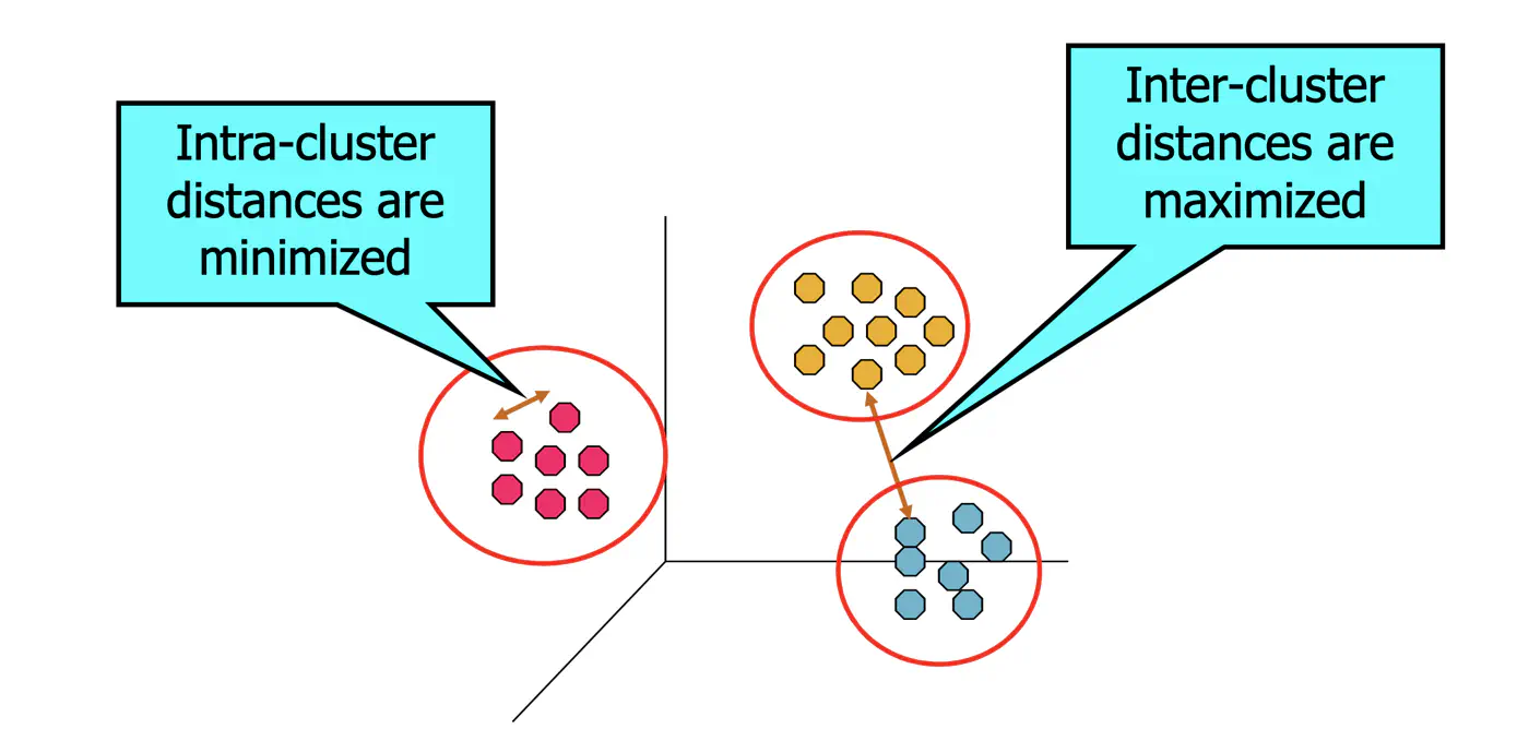
Such that points within clusters are ‘similar’.
And points across clusters are ‘dissimilar’.
This is fundamentally an optimization problem, i.e, find parameters such that the value is minimum/maximum. We need:
- An objective function
- what makes a clustering ‘good’?
- An algorithm to optimize it
- how do we find good clusters?
- Evaluation metrics
- how do we measure quality?
Objective function:
👉Minimize the within-cluster sum of squares (WCSS).
- Where:
- C = {C₁, …, Cₖ} are cluster assignments.
- μⱼ is the centroid (mean) of cluster Cₖ.
- ||·||² is squared Euclidean distance.
Note: Every point belongs to one and only one cluster.
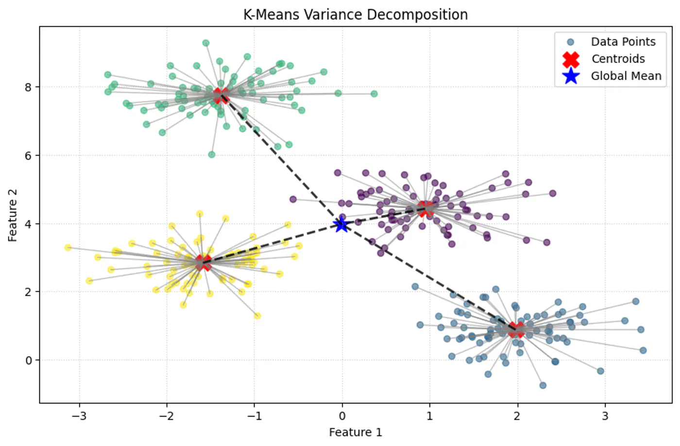
💡Within-Cluster Sum of Squares (WCSS) is nothing but variance.
⭐️ Total Variance = Within-Cluster Variance + Between-Cluster Variance
👉K-Means minimizes within-Cluster variance, which implicitly maximizes between-cluster separation.
Geometric Interpretation:
- Each point is ‘pulled’ toward its cluster center.
- The objective measures total squared distance of all points to their centers.
- Lower J(C, μ) means tighter, more compact clusters.
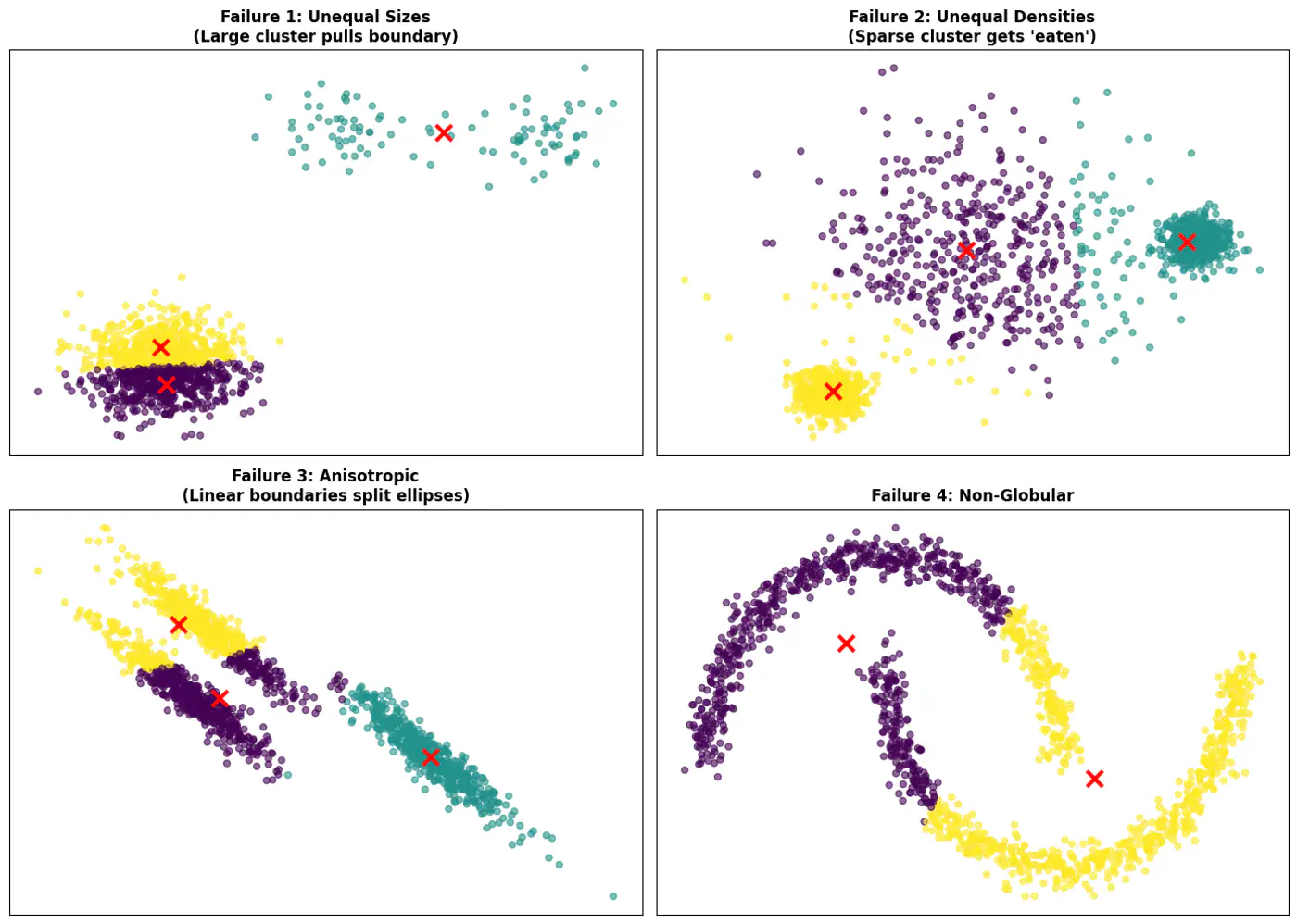
Note: K-Means works best when clusters are roughly spherical, similarly sized, and well-separated.
⭐️The problem requires partitioning ’n’ observations into ‘k’ distinct, non-overlapping clusters, which is given by the Stirling number of the second kind, which grows at a rate roughly equal to \(k^n/k!\).
\[S(n,k)=\frac{1}{k!}\sum _{j=0}^{k}(-1)^{k-j}{k \choose j}j^{n}\]\[S(100,2)=2^{100-1}-1=2^{99}-1\]\[2^{99}\approx 6.338\times 10^{29}\]👉This large number of possible combinations makes the problem NP-Hard.
🦉The k-means optimization problem is NP-hard because it belongs to a class of problems for which no efficient (polynomial-time ⏰) algorithm is known to exist.
End of Section
1.2 - Lloyds Algorithm
Iterative method for partitioning ’n’ data points into ‘k’ groups by repeatedly assigning data points to the nearest centroid (mean) and then recalculating centroids until assignments stabilize, aiming to minimize within-cluster variance.
📥Input: X = {x₁, …, xₙ}, ‘k’ (number of clusters)
📤Output: ‘C’ (clusters), ‘μ’ (centroids)
👉Steps:
- Initialize: Randomly choose ‘k’ cluster centroids μ₁, …, μₖ.
- Repeat until convergence, i.e, until cluster assignments and centroids no longer change significantly.
- a) Assignment: Assign each data point to the cluster whose centroid is closest (usually using Euclidean distance).
- For each point xᵢ: cᵢ = argminⱼ ||xᵢ - μⱼ||²
- b) Update: Recalculate the centroid (mean) of each cluster.
- For each cluster j: μⱼ = (1/|Cⱼ|) Σₓᵢ∈Cⱼ xᵢ
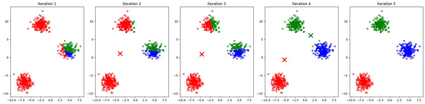
- Initialization sensitive, different initialization may lead to different clusters.
- Tries to make each cluster of same size that may not be the case in real world.
- Tries to make each cluster with same density(variance)
- Does not work well with non-globular(spherical) data.
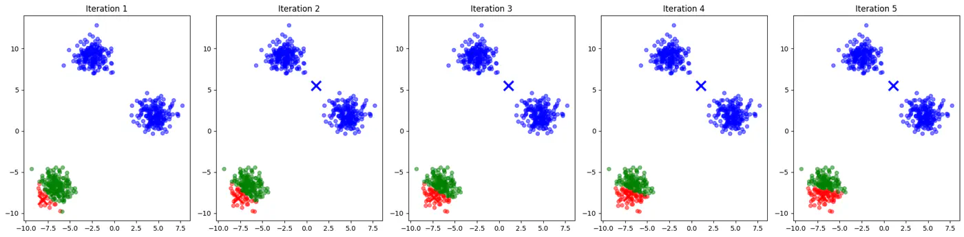
👉See how 2 different runs of K-Means algorithm gives totally different clusters.

👉Also, K-Means does not work well with non-spherical clusters, or clusters with different densities and sizes.
✅ Do not select initial points randomly, but some logic, such as, K-means++ algorithm.
✅ Use hierarchical clustering or density based clustering DBSCAN.
End of Section
1.3 - K Means++
- If two initial centroids belong to the same natural cluster, the algorithm will likely split that natural cluster in half and be forced to merge two other distinct clusters elsewhere to compensate.
- Inconsistent; different runs may lead to different clusters.
- Slow convergence; Centroids may need to travel much farther across the feature space, requiring more iterations.
👉Example for different K-Means algorithm runs give different clusters

💡Addresses the issue due to random initialization by aiming to spread out the initial centroids across the data points.
Steps:
- Select the first centroid: Choose one data point randomly from the dataset to be the first centroid.
- Calculate distances: For every data point x not yet selected as a centroid, calculate the distance, D(x), between x and the nearest centroid chosen so far.
- Select the next centroid: Choose the next centroid from the remaining data points with a probability
proportional to D(x)^2.
This makes it more likely that a point far from existing centroids is selected, ensuring the initial centroids are well-dispersed. - Repeat: Repeat steps 2 and 3 until ‘k’ number of centroids are selected.
- Run standard K-means: Once the initial centroids are chosen, the standard k-means algorithm proceeds with assigning data points to the nearest centroid and iteratively updating the centroids until convergence.
End of Section
1.4 - K Medoid
- In K-Means, the centroid is the arithmetic mean of the cluster. The mean is very sensitive to outliers.
- Not interpretable; centroid is the mean of cluster data points and may not be an actual data point, hence not representative.
⭐️Medoid is a specific data point from a dataset that acts as the ‘center’ or most representative member of its cluster.
👉It is defined as the object within a cluster whose average dissimilarity (distance) to all other members in that same cluster is the smallest.
💡Selects actual data points from the dataset as cluster representatives, called medoids (most centrally located).
👉a.k.a Partitioning Around Medoids(PAM).
Steps:
- Initialization: Select ‘k’ data points from the dataset as the initial medoids using K-Means++ algorithm.
- Assignment: Calculate the distance (e.g., Euclidean or Manhattan) from each non-medoid point to all medoids and assign each point to the cluster of its nearest medoid.
- Update (Swap):
- For each cluster, swap current medoid with a non-medoid point from the same cluster.
- For each swap, calculate the total cost 💰(sum of distances from medoid).
- Pick the medoid with minimum cost 💰.
- Repeat🔁: Repeat the assignment and update steps until (convergence), i.e, medoids no longer change or a maximum number of iterations is reached.
Note: Kind of brute-force algorithm, computationally expensive for large dataset.
✅ Flexible Distance Metrics: It can work with any dissimilarity measure (Manhattan, Cosine similarity), making it ideal for categorical or non-Euclidean data.
✅ Interpretable Results: Cluster centers are real observations (e.g., a ‘typical’ customer profile), which makes the output easier to explain to stakeholders.
End of Section
1.5 - Clustering Quality Metrics
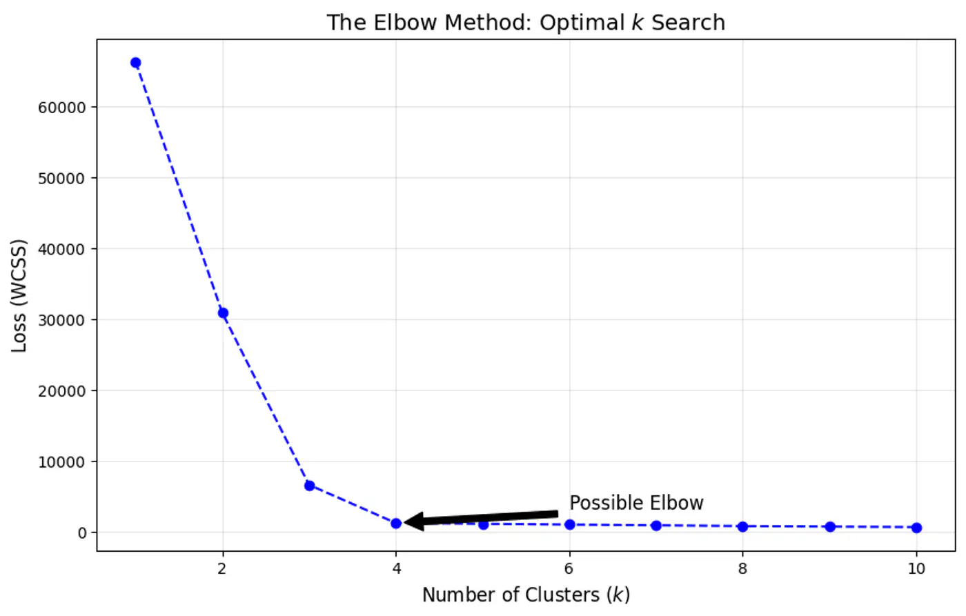
- 👉 Elbow Method: Quickest to compute; good for initial EDA (Exploratory Data Analysis).
- 👉 Dunn Index: Focuses on the ‘gap’ between the closest clusters.
- 👉 Silhouette Score: Balances compactness and separation.
- 👉 Domain specific knowledge and system constraints.
⭐️Heuristic used to determine the optimal number of clusters (k) for clustering by visualizing how the quality of clustering improves as ‘k’ increases.
🎯The goal is to find a value of ‘k’ where adding more clusters provides a diminishing return in terms of variance reduction.
⭐️Clustering quality evaluation metric that measures: separation (between clusters) and compactness (within clusters)
Note: A higher Dunn Index value indicates better clustering, meaning clusters are well-separated from each other and compact.
👉Dunn Index Formula:
\[DI = \frac{\text{Minimum Inter-Cluster Distance(between different clusters)}}{\text{Maximum Intra-Cluster Distance(within a cluster)}}\]\[DI = \frac{\min_{1 \le i < j \le k} \delta(C_i, C_j)}{\max_{1 \le l \le k} \Delta(C_l)}\]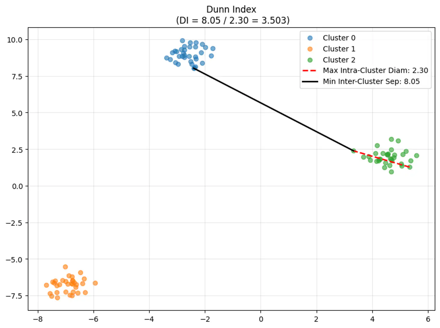
👉Let’s understand the terms in the above formula:
\(\delta(C_i, C_j)\) (Inter-Cluster Distance):
- Measures how ‘far apart’ the clusters are.
- Distance between the two closest points of different clusters (Single-Linkage distance). \[\delta(C_i, C_j) = \min_{x \in C_i, y \in C_j} d(x, y)\]
\(\Delta(C_l)\) (Intra-Cluster Diameter):
- Measures how ‘spread out’ a cluster is.
- Distance between the two furthest points within the same cluster (Complete-Linkage distance). \[\Delta(C_l) = \max_{x, y \in C_l} d(x, y)\]
- Single Linkage (MIN): Uses the minimum distance between any two points in different clusters.
- Complete Linkage (MAX): Uses the maximum distance between any two points in same cluster.
End of Section
1.6 - Silhouette Score
- ✅ Elbow Method: Quickest to compute; good for initial EDA.
- ✅ Dunn Index: Focuses on the ‘gap’ between the closest clusters.
——- We have seen the above 2 methods in the previous section ———- - 👉 Silhouette Score: Balances compactness and separation.
- 👉 Domain specific knowledge and system constraints.
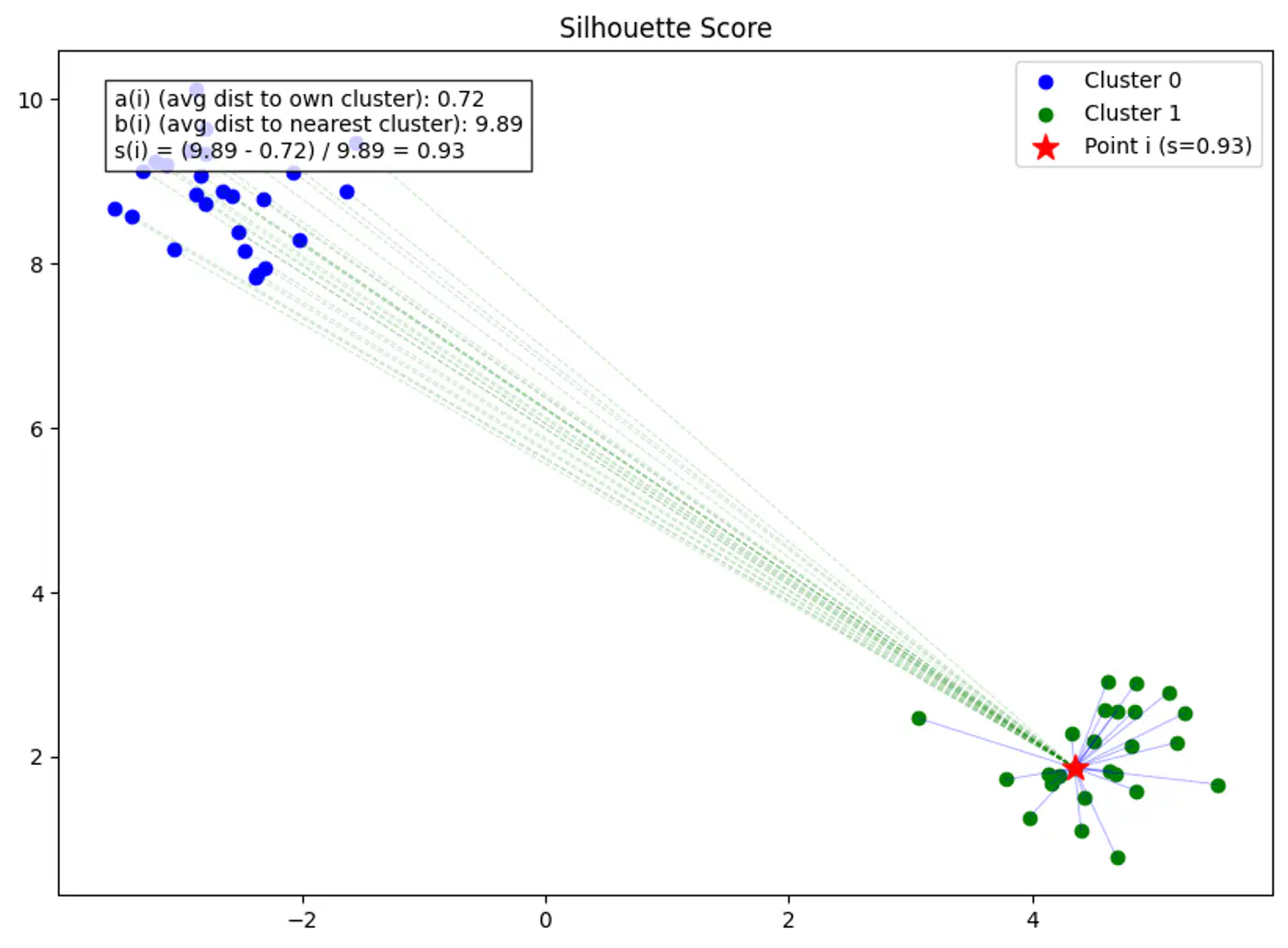
⭐️Clustering quality evaluation metric that measures how similar a data point is to its own cluster (cohesion) compared to other clusters (separation).
Note: Higher scores (closer to 1) indicate better-defined, distinct clusters, while scores near 0 suggest overlapping clusters, and negative scores mean points might be in the wrong cluster.
Silhouette score for point ‘i’ is the difference between separation b(i) and cohesion a(i), normalized by the larger of the two.
\[ s(i) = \frac{b(i) - a(i)}{\max(a(i), b(i))} \]Note: The Global Silhouette Score is simply the mean of s(i) for all points in the dataset.
👉Example for Silhouette Score:
👉Example for Silhouette Score of 0(Border Point) and negative(Wrong Cluster).
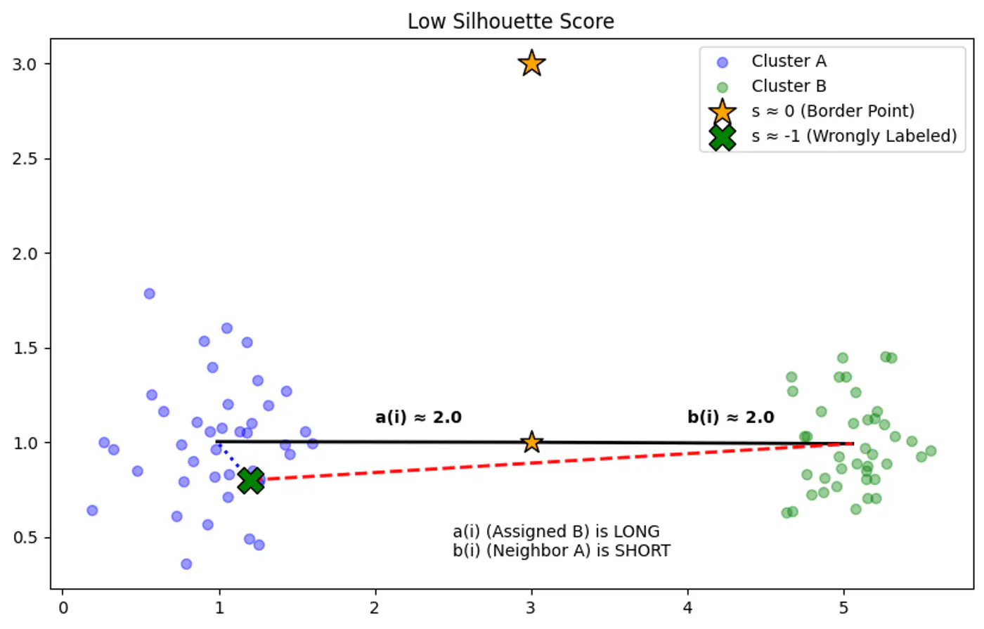
🦉Now let’s understand the terms in Silhouette Score in detail.
Average distance between point ‘i’ and all other points in the same cluster.
\[a(i) = \frac{1}{|C_A| - 1} \sum_{j \in C_A, i \neq j} d(i, j)\]Note: Lower a(i) means the point is well-matched to its own cluster.
Average distance between point ‘i’ and all points in the nearest neighboring cluster (the cluster that ‘i’ is not a part of, but is closest to).
\[b(i) = \min_{C_B \neq C_A} \frac{1}{|C_B|} \sum_{j \in C_B} d(i, j)\]Note: Higher b(i) means the point is very far from the next closest cluster.
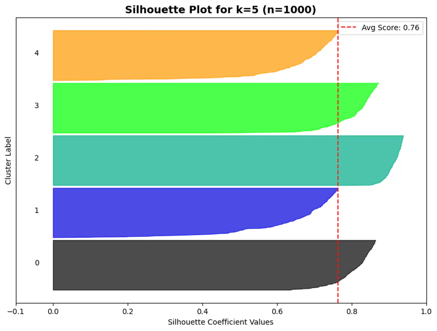
⭐️A silhouette plot is a graphical tool used to evaluate the quality of clustering algorithms (like K-Means), showing how well each data point fits within its cluster.
👉Each bar gives the average silhouette score of the points assigned to that cluster.
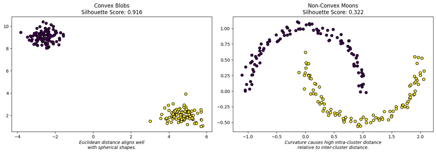
⛳️ Like K-Means, the Silhouette Score (when using Euclidean distance) assumes convex clusters.
🌘 If we use it on ‘Moon’ shaped clusters, it will give a low score even if the clusters are perfectly separated, because the ‘average distance’ to a neighbor might be small due to the curvature of the manifold.
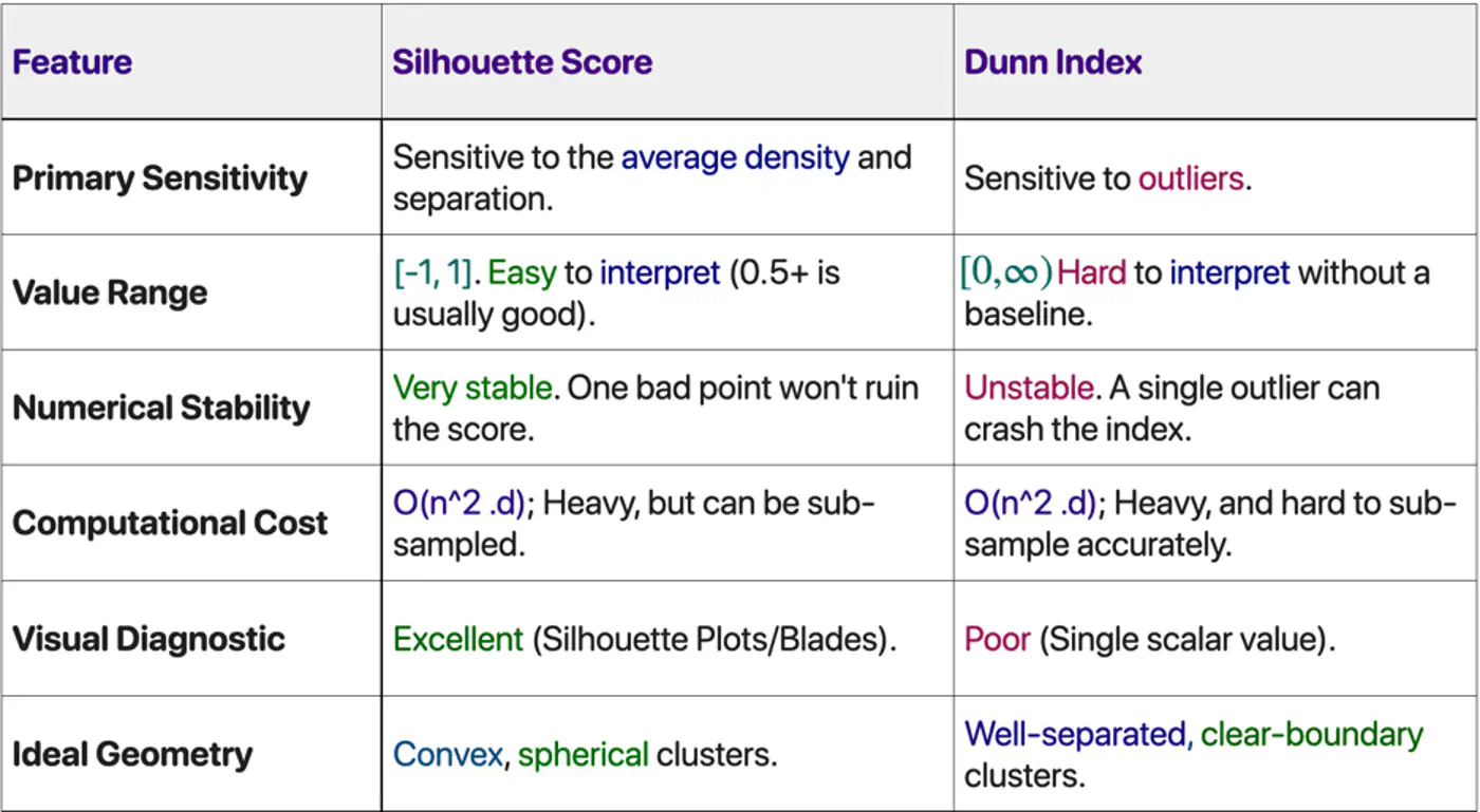
Choose Silhouette Score if:
✅ Need a human-interpretable metric to present to stakeholders.
✅ Dealing with real-world noise and overlapping ‘fuzzy’ boundaries.
✅ Want to see which specific clusters are weak (using the plot).
Choose Dunn Index if:
✅ Performing ‘Hard Clustering’ where separation is a safety or business requirement.
✅ Data is pre-cleaned of outliers (e.g., in a curated embedding space).
✅ Need to compare different clustering algorithms (e.g., K-Means vs. DBSCAN) on a high-integrity task.
End of Section
2 - Hierarchical Clustering
2.1 - Hierarchical Clustering
- 🤷 We might not know in advance the number of distinct clusters ‘k’ in the dataset.
- 🕸️ Also, sometimes the dataset may contain a nested structure or some inherent hierarchy, such as, file system, organizational chart, biological lineages, etc.
⭐️ Method of cluster analysis that seeks to build a hierarchy of clusters, resulting in a tree like structure called dendrogram.
👉Hierarchical clustering allows us to explore different possibilities (of ‘k’) by cutting the dendrogram at various levels.
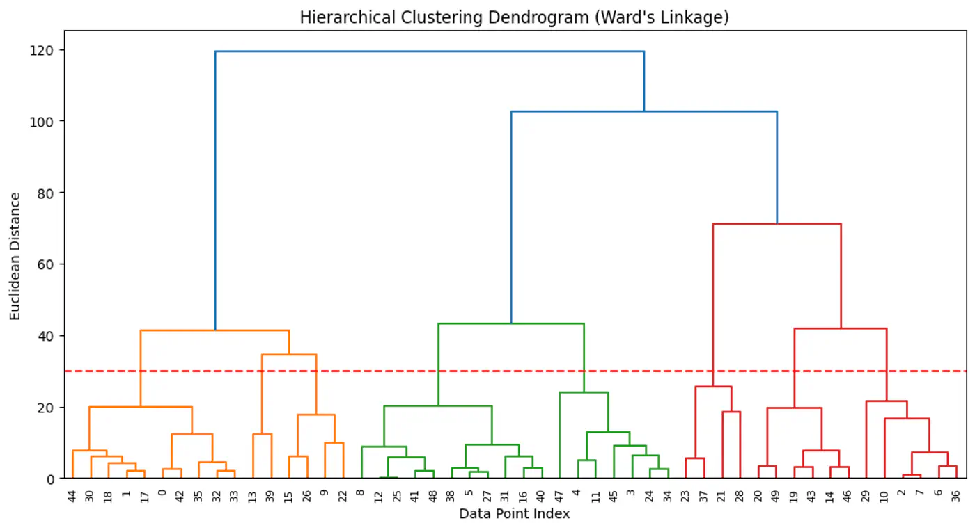
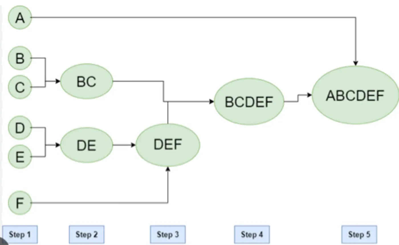
Agglomerative (Bottom-Up):
Most common, also known as Agglomerative Nesting (AgNes).
- Every data point starts as its own cluster.
- In each step, merge the two ‘closest’ clusters.
- Repeat step 2, until all points are merged in a single cluster.
Divisive (Top-Down):
- All data points start in one large cluster.
- In each step, divide the cluster into two halves.
- Repeat step 2, until every point is its own cluster.
Agglomerative Clustering Example:
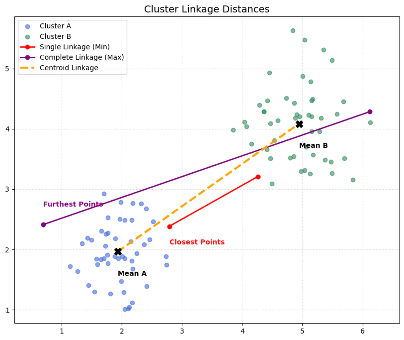
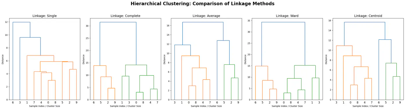
- Ward’s Method:
- Merges clusters to minimize the increase in the total within-cluster variance (sum of squared errors), resulting in compact, equally sized clusters.
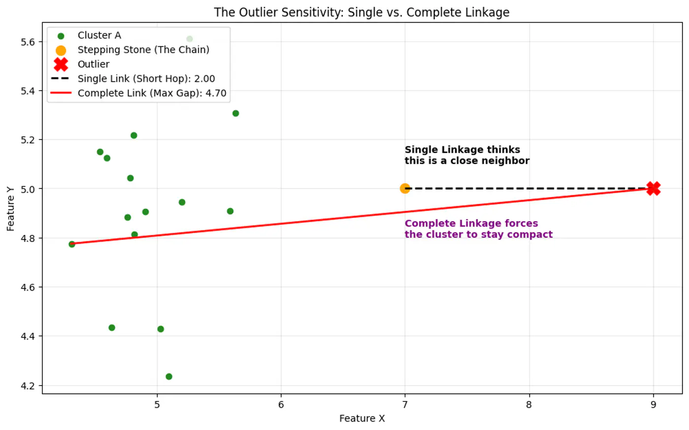
- Single Linkage (MIN):
- Uses the minimum distance between any two points in different clusters.
- Prone to creating long, ‘chain-like’ 🔗 clusters, sensitive to outliers.
- Complete Linkage (MAX):
- Uses the maximum distance between any two points in different clusters.
- Forms tighter, more spherical clusters, less sensitive to outliers than single linkage.
- Average Linkage:
- Combines clusters by the average distance between all points in two clusters, offering a compromise between single and complete linkage.
- A good middle ground, often overcoming limitations of single and complete linkage.
- Centroid Method:
- Merges clusters based on the distance between their centroids (mean points).
👉Single Linkage is more sensitive to outlier than Complete Linkage, as Single Linkage can keep linking to the closest point forming a bridge to outlier.
👉All cluster linkage distances.
👉We get different clustering using different linkages.
End of Section
3 - DBSCAN
3.1 - DBSCAN
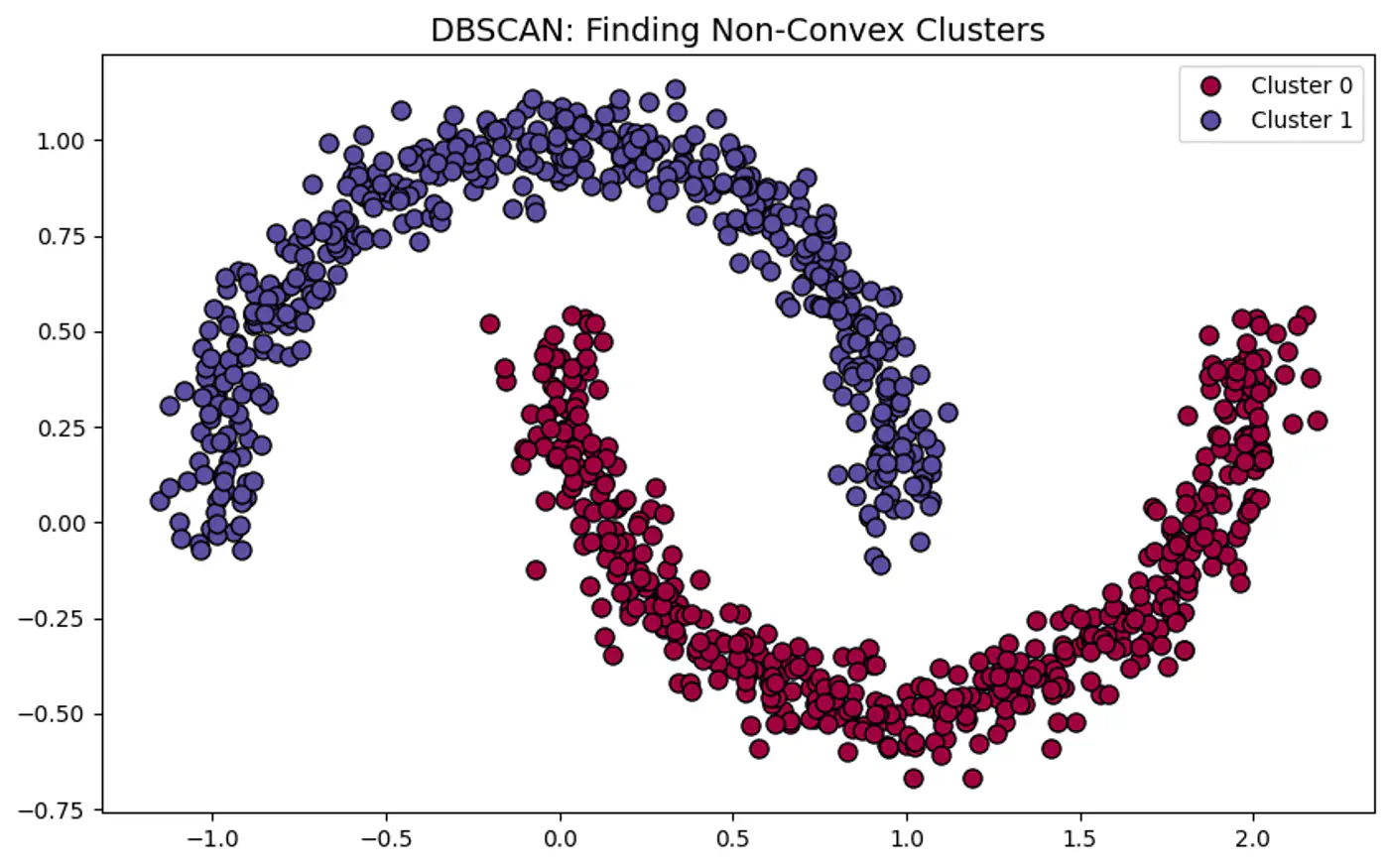
- Non-Convex Shapes: K-Means can not find ‘crescent’ or ‘ring’ shape clusters.
- Noise: K-Means forces every point into a cluster, even outliers.
👉K-Means asks:
- “Which center is closest to this point?”
👉DBSCAN asks:
- “Is this point part of a dense neighborhood?”
⭐️Groups closely packed data points into clusters based on their density, and marks points that lie alone in low-density regions as outliers or noise.
Note: Unlike K-means, DBSCAN can find arbitrarily shaped clusters and does not require the number of clusters to be specified beforehand.
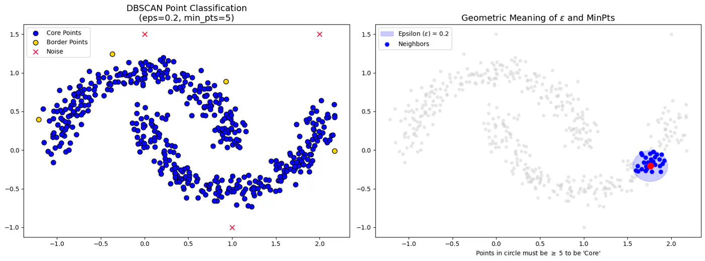
- Epsilon (eps or \(\epsilon\)):
- Radius that defines the neighborhood around a data point.
- If it’s too small, many points will be noise, and if too large, distinct clusters may merge.
- Minimum Points(minPts or min_samples):
- Minimum number of data points required within a point’s -neighborhood for that point to be considered a dense region (a core point).
- Defines threshold for ‘density’.
- Rule of thumb: minPts dimensions + 1; use larger value for noisy data (minPts 2*dimensions).
- Core Point:
- If it has at least minPts (including itself) within its -neighborhood.
- Forms the dense backbone of the clusters and can expand them.
- Border Point:
- If it has at fewer than minPts within its -neighborhood but falls within the -neighborhood of a core point.
- Border points belong to a cluster but cannot expand it further.
- Noise Point (Outlier):
- If it is neither a core point nor a border point, i.e., it is not density-reachable from any core point.
- Not assigned to any cluster.
- Random Start:
- Mark all points as unvisited; pick an arbitrary unvisited point ‘P’ from the dataset.
- Density Check:
- Check the point P’s ϵ-neighborhood.
- If ‘P’ has at least minPts, it is identified as a core point, and a new cluster is started.
- If it has fewer than minPts, the point is temporarily labeled as noise (it might become a border point later).
- Cluster Expansion:
- Recursively visit all points in P’s ϵ-neighborhood.
- If they are also core points, their neighbors are added to the cluster.
- Iteration 🔁:
- This ‘density-reachable’ logic continues until the cluster is fully expanded.
- The algorithm then picks another unvisited point and repeats the process, discovering new clusters or marking more points as noise until all points are processed.
👉DBSCAN can correctly detect non-spherical clusters.
👉DBSCAN Points and Epsilon-Neighborhood.
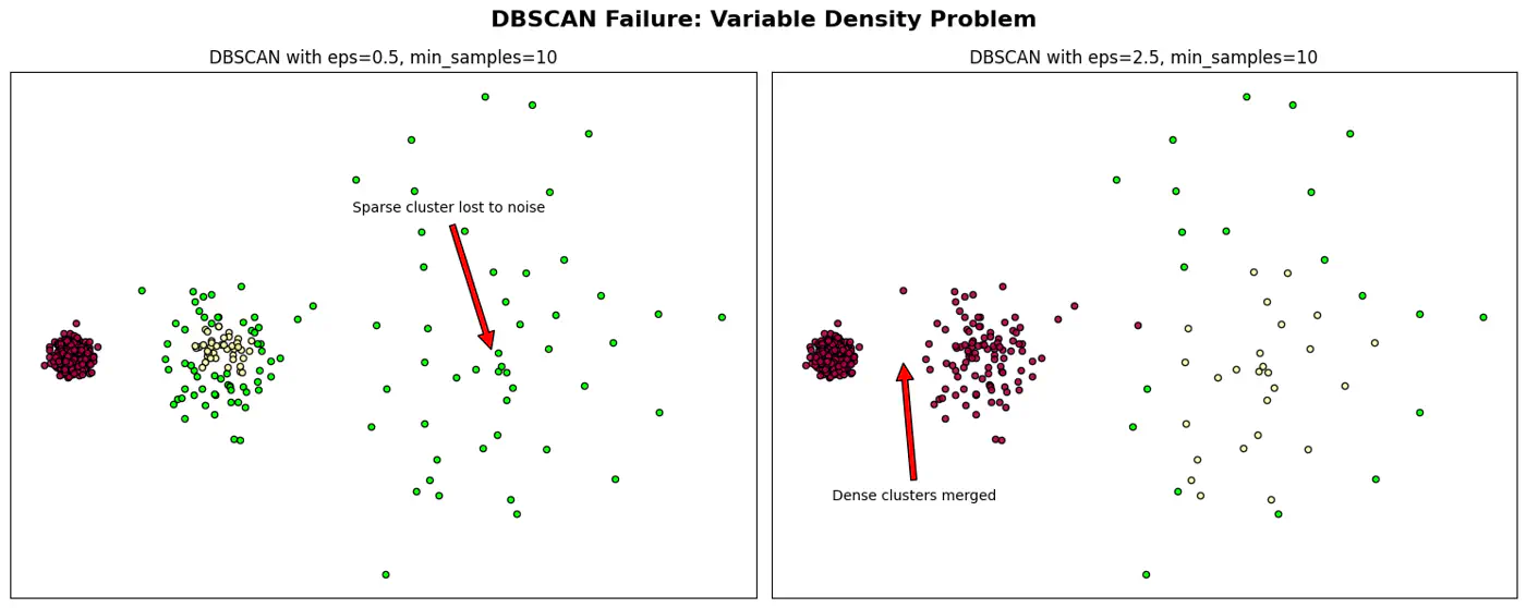
- Varying Density Clusters:
- Say A cluster is very dense and B is sparse, a single cannot satisfy both clusters.
- High Dimensional Data:
- ‘Curse of Dimensionality’ - In high-dimensional space, the distance between any two points converge.
Note: Sensitive to parameter eps and minPts; tricky to get it work.
👉DBSCAN Failure and Epsilon ((\epsilon)
Arbitrary Cluster Shapes:
- When clusters are intertwined, nested, or ‘moon-shaped’; where K-Means would fail by splitting them.
Presence of Noise and Outliers:
- Robust to noise and outliers because it explicitly identifies low-density points as noise (labeled as -1) rather than forcing them into a cluster.
End of Section
4 - Gaussian Mixture Model
4.1 - Gaussian Mixture Models
- K-means uses Euclidean distance and assumes that clusters are spherical (isotropic) and have the same variance across all dimensions.
- Places a circle or sphere around each centroid.
- What if the clusters are elliptical ? 🤔
👉K-Means Fails with Elliptical Clusters.
💡GMM: ‘Probabilistic evolution’ of K-Means
⭐️ GMM provides soft assignments and can model elliptical clusters by accounting for variance and correlation between features.
Note: GMM assumes that all data points are generated from a mixture of a finite number of Gaussian Distributions with unknown parameters.
👉GMM can Model Elliptical Clusters.
💡‘Combination of probability distributions’.
👉Soft Assignment: Instead of a simple ‘yes’ or ’no’ for cluster membership, a data point is assigned a set of probabilities, one for each cluster.
e.g: A data point might have a 60% probability of belonging to cluster ‘A’, 30% probability for cluster ‘B’, and 10% probability for cluster ‘C’.
👉Gaussian Mixture Model Example:
Note: The term \(1/(\sqrt{2\pi \sigma ^{2}})\) is a normalization constant to ensure the total area under the curve = 1.
👉Multivariate Gaussian Example:

Whenever we have multivariate Gaussian, then the variables may be independent or correlated.
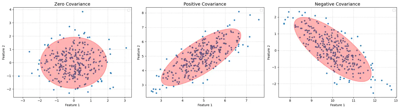
👉Feature Covariance:
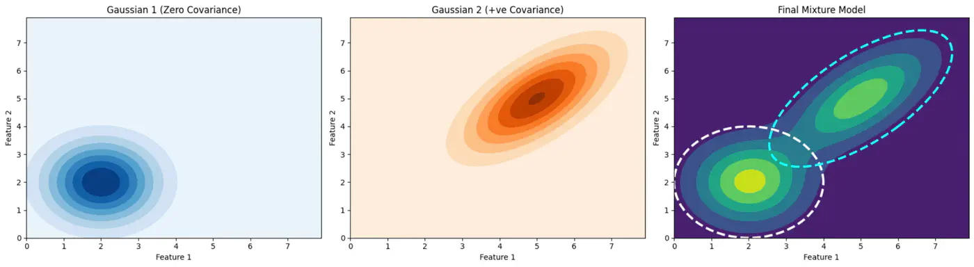
👉Gaussian Mixture with PDF
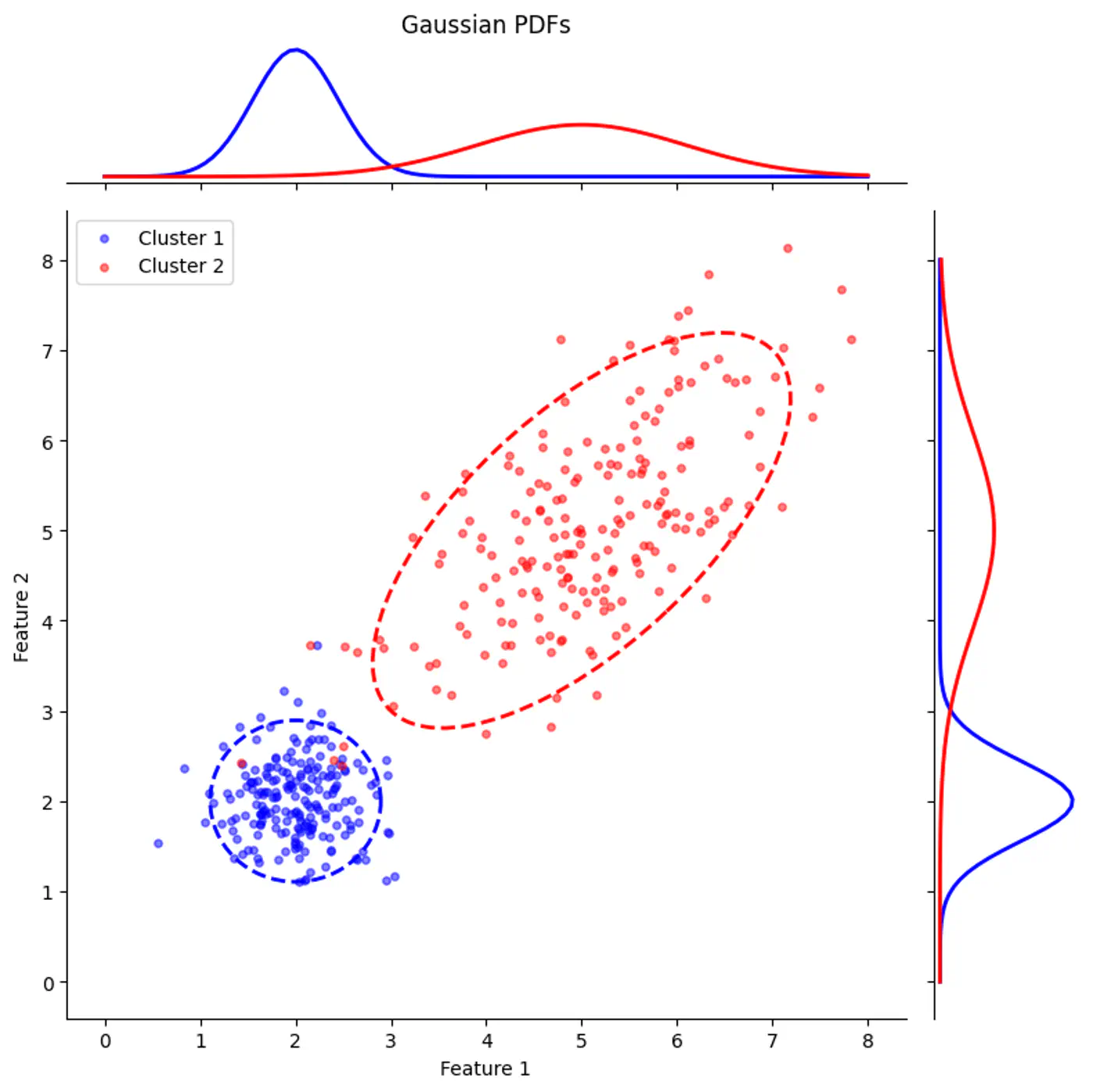
👉Gaussian Mixture (2D)
End of Section
4.2 - Latent Variable Model
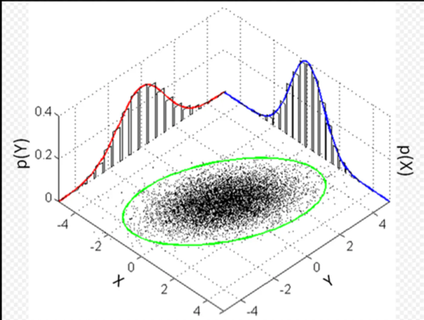
⭐️Probabilistic model that assumes data is generated from a mixture of several Gaussian (normal) distributions with unknown parameters.
🎯GMM represents the probability density function of the data as a weighted sum of ‘K’ component Gaussian densities.
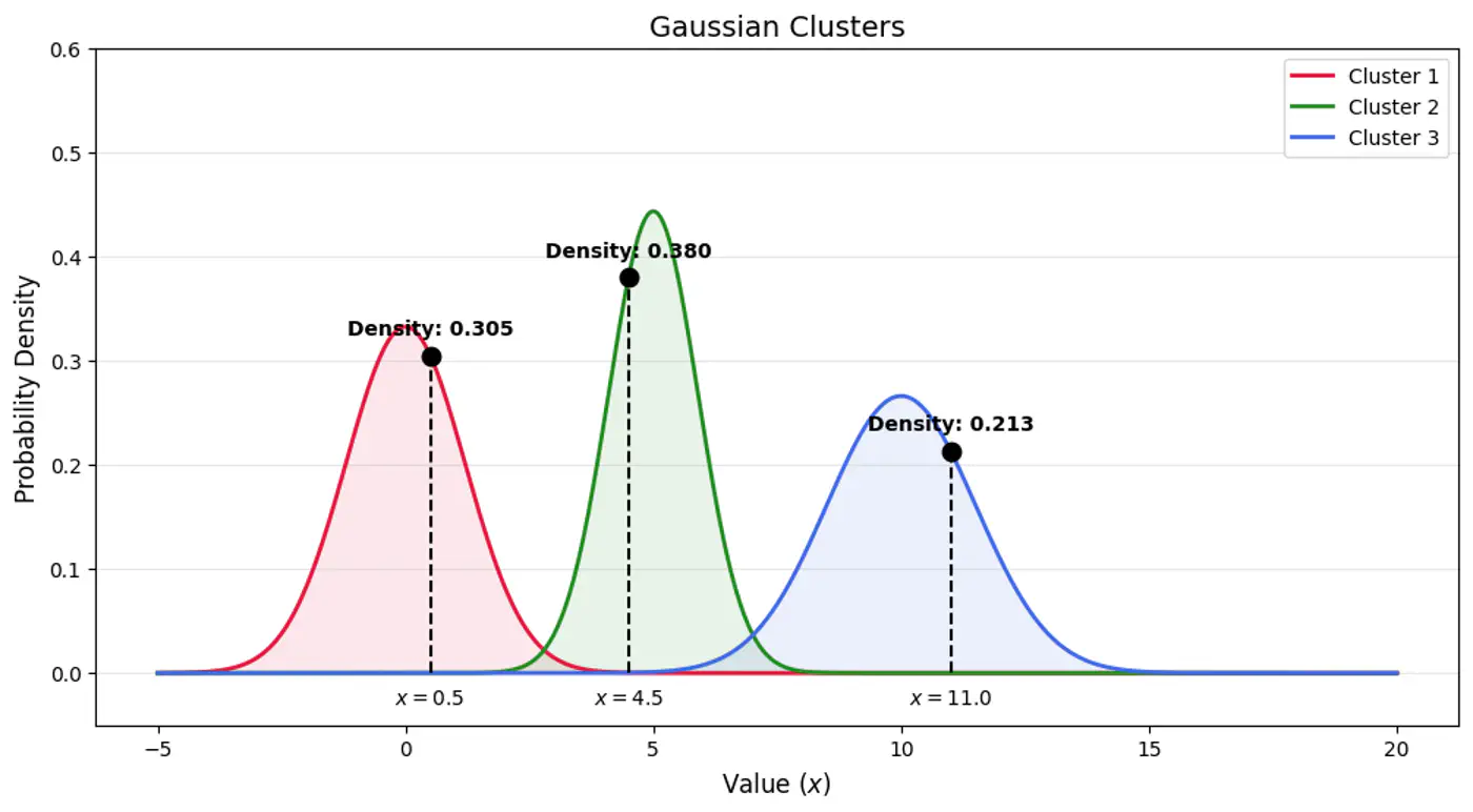
👉Below plot shows the probability of a point being generated by 3 different Gaussians.
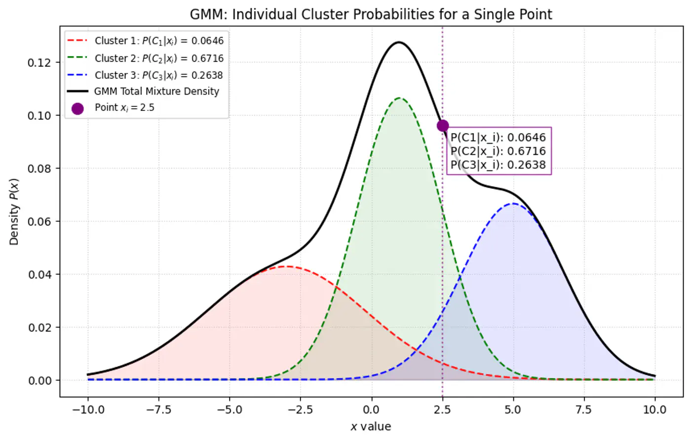
Overall density \(p(x_i|\mathbf{\theta })\) for a data point ‘\(x_i\)’:
\[p(x_i|\mathbf{\mu},\mathbf{\Sigma} )=\sum _{k=1}^{K}\pi _{k}\mathcal{N}(x_i|\mathbf{\mu }_{k},\mathbf{\Sigma }_{k})\]- K: number of component Gaussians.
- \(\pi_k\): mixing coefficient (weight) of the k-th component, such that, \(\pi_k \ge 0\) and \(\sum _{k=1}^{K}\pi _{k}=1\).
- \(\mathcal{N}(x_i|\mathbf{\mu }_{k},\mathbf{\Sigma }_{k})\): probability density function of the k-th Gaussian component with mean \(\mu_k\) and covariance matrix \(\Sigma_k\).
- \(\mathbf{\theta }=\{(\pi _{k},\mathbf{\mu }_{k},\mathbf{\Sigma }_{k})\}_{k=1}^{K}\): complete set of parameters to be estimated.
Note: \(\pi _{k}\approx \frac{\text{Number\ of\ points\ in\ cluster\ }k}{\text{Total\ number\ of\ points\ }(N)}\)
👉 Weight of the cluster is proportional to the number of points in the cluster.
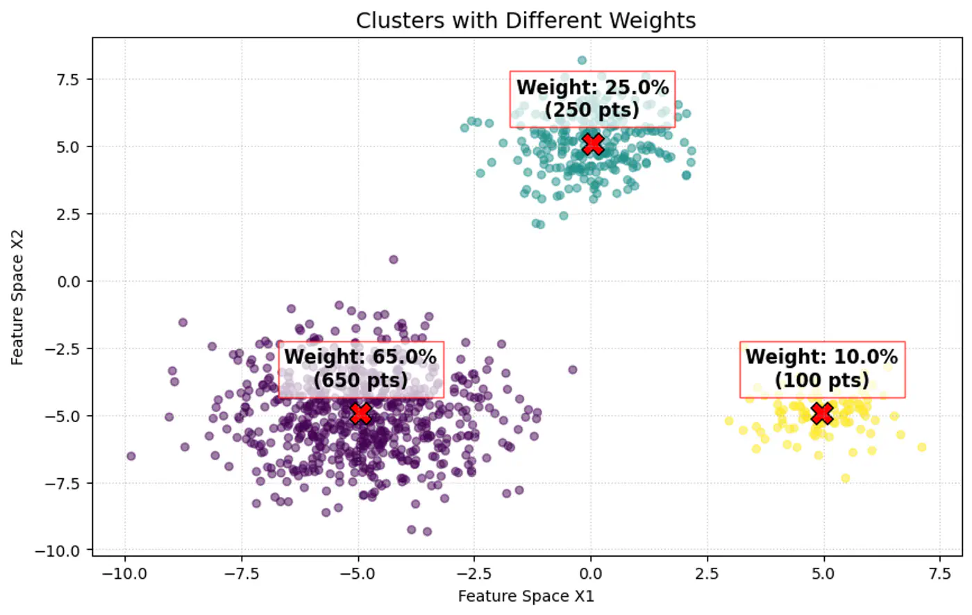
👉Below image shows the weighted Gaussian PDF, given the weights of clusters.
🎯 Goal of a GMM optimization is to find the set of parameters \(\Theta =\{(\pi _{k},\mu _{k},\Sigma _{k})\mid k=1,\dots ,K\}\) that maximize the likelihood of observing the given data.
\[L(\Theta |X)=\sum _{i=1}^{N}\log P(x_i|\Theta )=\sum _{i=1}^{N}\log \left(\sum _{k=1}^{K}\pi _{k}\mathcal{N}(x_i|\mu _{k},\Sigma _{k})\right)\]- 🦀 \(\log (A+B)\) cannot be simplified.
- 🦉So, is there any other way ?
⭐️Imagine we are measuring the heights of people in a college.
- We see a distribution with two peaks (bimodal).
- We suspect there are two underlying groups:
- Group A (Men) and Group B (Women).
Observation:
- Observed Variable (X): Actual height measurements.
- Latent Variable (Z): The ‘label’ (Man or Woman) for each person.
Note: We did not record gender, so it is ‘hidden’ or ‘latent’.
⭐️GMM is a latent variable model, meaning each data point \(\mathbf{x}_{i}\) is assumed to have an associated unobserved (latent) variable \(z_{i}\in \{1,\dots ,K\}\) indicating which component generated it.
Note: We observe the data point, but we do not observe which cluster it belongs to (\(z_i\)).
👉If we knew the value of \(z_i\) (component indicator) for every point, estimating the parameters of each Gaussian component would be straightforward.
Note: The challenge lies in estimating both the parameters of the Gaussians and the values of the latent variables simultaneously.
- With ‘z’ unknown:
- maximize: \[ \log \sum _{k}\pi _{k}\mathcal{N}(x_{i}|\mu _{k},\Sigma _{k}) = \log \Big(\pi _{1}\mathcal{N}(x_{i}\mid \mu _{1},\Sigma _{1})+\pi _{2}\mathcal{N}(x_{i}\mid \mu _{2},\Sigma _{2})+ \dots + \pi _{k}\mathcal{N}(x_{i}\mid \mu _{k},\Sigma _{k})\Big)\]
- \(\log (A+B)\) cannot be simplified.
- maximize: \[ \log \sum _{k}\pi _{k}\mathcal{N}(x_{i}|\mu _{k},\Sigma _{k}) = \log \Big(\pi _{1}\mathcal{N}(x_{i}\mid \mu _{1},\Sigma _{1})+\pi _{2}\mathcal{N}(x_{i}\mid \mu _{2},\Sigma _{2})+ \dots + \pi _{k}\mathcal{N}(x_{i}\mid \mu _{k},\Sigma _{k})\Big)\]
- With ‘z’ known:
- The log-likelihood of the ‘complete data’ simplifies into a sum of logarithms:
\[\sum _{i}\log (\pi _{z_{i}}\mathcal{N}(x_{i}|\mu _{z_{i}},\Sigma _{z_{i}}))\]
- Every point is assigned to exactly one cluster, so the sum disappears because there is only one cluster responsible for that point.
- The log-likelihood of the ‘complete data’ simplifies into a sum of logarithms:
\[\sum _{i}\log (\pi _{z_{i}}\mathcal{N}(x_{i}|\mu _{z_{i}},\Sigma _{z_{i}}))\]
Note: This allows the logarithm to act directly on the exponential term of the Gaussian, leading to simple linear equations.
👉When ‘z’ is known, every data point is ‘labeled’ with its parent component.
To estimate the parameters (mean \(\mu_k\) and covariance \(\Sigma_k\)) for a specific component ‘k’ :
- Gather all data points \(x_i\), where \(z_i\)= k.
- Calculate the standard Maximum Likelihood Estimate.(MLE) for that single Gaussian using only those points.
⭐️ Knowing ‘z’ provides exact counts and component assignments, leading to direct formulae for the parameters:
- Mean (\(\mu_k\)): Arithmetic average of all points assigned to component ‘k’.
- Covariance (\(\Sigma_k\)): Sample covariance of all points assigned to component ‘k’.
- Mixing Weight (\(\pi_k\)): Fraction of total points assigned to component ‘k’.
End of Section
4.3 - Expectation Maximization
- If we knew the parameters (\(\mu, \Sigma, \pi\)) we could easily calculate which cluster ‘z’ each point belongs to (using probability).
- If we knew the cluster assignments ‘z’ of each point, we could easily calculate the parameters for each cluster (using simple averages).
🦉But we do not know either of them, as the parameters of the Gaussians - we aim to find and cluster indicator latent variable is hidden.

⛳️ Find latent cluster indicator variable \(z_{ik}\).
But \(z_{ik}\) is a ‘hard’ assignment’ (either ‘0’ or ‘1’).
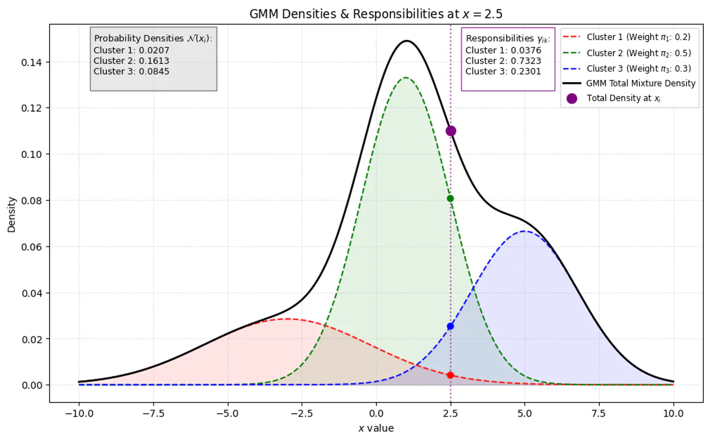
- 🦆 Because we do not observe ‘z’, we use another variable ‘Responsibility’ (\(\gamma_{ik}\)) as a ‘soft’ assignment (value between 0 and 1).
- 🐣 \(\gamma_{ik}\) is the expected value of the latent variable \(z_{ik}\), given the observed data \(x_{i}\) and parameters \(\Theta\). \[\gamma _{ik}=E[z_{ik}\mid x_{i},\theta ]=P(z_{ik}=1\mid x_{i},\theta )\]
Note: \(\gamma_{ik}\) is the posterior probability (or ‘responsibility’) that cluster ‘k’ takes for explaining data point \(x_{i}\).
⭐️Using Bayes’ Theorem, we derive responsibility (posterior probability that component ‘k’ generated data point \(x_i\)) by combining the prior/weights (\(\pi_k\)) and the likelihood (\(\mathcal{N}(x_{i}\mid \mu _{k},\Sigma _{k})\)).
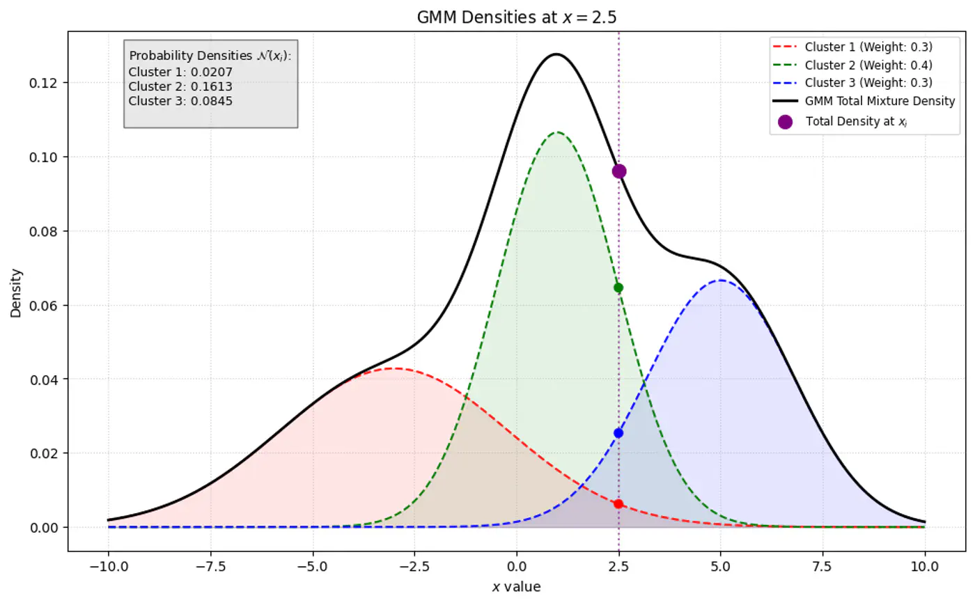
\[\gamma _{ik}= P(z_{ik}=1\mid x_{i},\theta ) = \frac{P(z_{ik}=1)P(x_{i}\mid z_{ik}=1)}{P(x_{i})}\]\[\gamma _{ik}=\frac{\pi _{k}\mathcal{N}(x_{i}\mid \mu _{k},\Sigma _{k})}{\sum _{j=1}^{K}\pi _{j}\mathcal{N}(x_{i}\mid \mu _{j},\Sigma _{j})}\]👉Bayes’ Theorem: \(P(A|B)=\frac{P(B|A)\cdot P(A)}{P(B)}\)
👉 GMM Densities at point
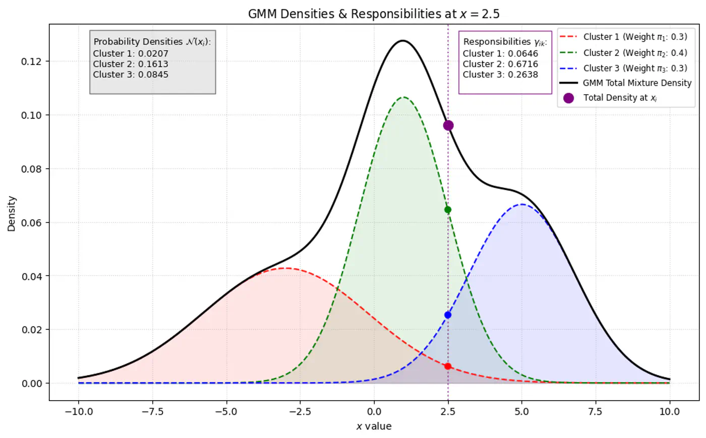
👉GMM Densities at point (different cluster weights)
- Initialization: Assign initial values to parameters (\(\mu, \Sigma, \pi\)), often using K-Means results.
- Expectation Step (E): Calculate responsibilities; provides ‘soft’ assignments of points to clusters.
- Maximization Step (M): Update parameters using responsibilities as weights to maximize the expected log-likelihood.
- Convergence: Repeat ‘E’ and ‘M’ steps until the change in log-likelihood falls below a threshold.
👉Given our current guess of the clusters, what is the probability that point \(x_i\) came from cluster ‘k’ ?
\[\gamma (z_{ik})=p(z_{i}=k|\mathbf{x}_{i},\mathbf{\theta }^{(\text{old})})=\frac{\pi _{k}^{(\text{old})}\mathcal{N}(\mathbf{x}_{i}|\mathbf{\mu }_{k}^{(\text{old})},\mathbf{\Sigma }_{k}^{(\text{old})})}{\sum _{j=1}^{K}\pi _{j}^{(\text{old})}\mathcal{N}(\mathbf{x}_{i}|\mathbf{\mu }_{j}^{(\text{old})},\mathbf{\Sigma }_{j}^{(\text{old})})}\]\(\pi_k\) : Probability that a randomly selected data point \(x_i\) belongs to the k-th component before we even look at the specific value of \(x_i\), such that \(\pi_k \ge 0\) and \(\sum _{k=1}^{K}\pi _{k}=1\).
👉Update the parameters (\(\mu, \Sigma, \pi\)) by calculating weighted versions of the standard MLE formulas using responsibilities as weight 🏋️♀️.
\[ \begin{align*} &\bullet \mathbf{\mu }_{k}^{(\text{new})}=\frac{1}{N_{k}}\sum _{i=1}^{N}\gamma (z_{ik})\mathbf{x}_{i} \\ &\bullet \mathbf{\Sigma }_{k}^{(\text{new})}=\frac{1}{N_{k}}\sum _{i=1}^{N}\gamma (z_{ik})(\mathbf{x}_{i}-\mathbf{\mu }_{k}^{(\text{new})})(\mathbf{x}_{i}-\mathbf{\mu }_{k}^{(\text{new})})^{\top } \\ &\bullet \pi _{k}^{(\text{new})}=\frac{N_{k}}{N} \end{align*} \]- where, \(N_{k}=\sum _{i=1}^{N}\gamma (z_{ik})\) is the effective number of points assigned to component ‘k'.
End of Section
5.1 - Anomaly Detection
🦄 Anomaly is a rare item, event or observation which deviates significantly from the majority of the data and does not conform to a well-defined notion of normal behavior.
Note: Such examples may arouse suspicions of being generated by a different mechanism, or appear inconsistent with the remainder of that set of data.
❌ Remove Outliers:
- Rejection or omission of outliers from the data to aid statistical analysis, for example to compute the mean or standard deviation of the dataset.
- Remove outliers for better predictions from models, such as linear regression.
🔦Focus on Outliers:
- Fraud detection in banking and financial services.
- Cyber-security: intrusion detection, malware, or unusual user access patterns.
- Supervised
- Semi-Supervised
- Unsupervised (most common) ✅
Note: Labeled anomaly data is often unavailable in real-world scenarios.
- Statistical Methods: Z-Score, large value means outlier, IQR, point beyond fences (Q1 - 1.5*IQR or Q3 + 1.5*IQR) is flagged as an outlier.
- Distance Based: KNN, points far from their neighbors as potential anomalies.
- Density Based: DBSCAN, points in low density regions are considered outliers.
- Clustering Based: K-Means, points far from cluster centroids that do not fit any cluster are anomalies.
- Elliptic Envelope (MCD - Minimum Covariance Determinant)
- One-Class SVM (OC-SVM)
- Local Outlier Factor (LOF)
- Isolation Forest (iForest)
- RANSAC (Random Sample Consensus)
End of Section
5.2 - Elliptic Envelope
Detect anomalies in multivariate Gaussian data, such as, biometric data (height/weight) where features are normally distributed and correlated.
Assumption: The data can be modeled by a Gaussian distribution.
In a normal distribution, most data points cluster around the mean, and the probability density decreases as we move farther away from the center.
🌍 Euclidean distance measures the simple straight-line distance from the center of the cloud.
👉If the data is spherical, this works fine.
🦕 However, real-world data is often stretched or skewed (e.g., taller people are generally heavier), due to correlations between variables, forming an elliptical shape.

⭐️Mahalanobis distance essentially re-scales the data so that the elliptical distribution appears spherical, and then measures the Euclidean distance in that transformed space.
👉This way, it measures how many standard deviations(\(\sigma\)) away a point is from the mean, considering the data’s spread and correlation (covariance).
\[D_M(x) = \sqrt{(x - \mu)^T \Sigma^{-1} (x - \mu)}\]👉Find the most dense core of the data.
\[D_M(x) = \sqrt{(x - \mu)^T \Sigma^{-1} (x - \mu)}\]🦣 Determinant of covariance matrix \(\Sigma\) represents the volume of the ellipsoid.
⏲️ Therefore, minimize \(|\Sigma|\) to find the tight core.
👉 \(\text {Small} ~ \Sigma \rightarrow \text {Large} ~\Sigma ^{-1}\rightarrow \text {Large} ~ D_{M} ~\text {for outliers}\)
MCD algorithm is used to find the covariance matrix \(\Sigma\) with minimum determinant, so that the volume of the ellipsoid is minimized.
- Initialization: Select several random subsets of size h < n (default h = \(\frac{n+d+1}{2}\), d = # dimensions), representing ‘robust’ majority of the data.
- Calculate preliminary mean (\(\mu\)) and covariance (\(\Sigma\)) for each random subset.
- Concentration Step: Iterative core of the algorithm designed to ‘tighten’ the ellipsoid.
- Calculate Distances: Compute the Mahalanobis distance of all ’n’ points in the dataset from the current subset’s mean (\(\mu\)) and covariance (\(\Sigma\)).
- Select New Subset: Identify the ‘h’ points with the smallest Mahalanobis distances.
- These are the points most centrally located relative to the current ellipsoid.
- Update Estimates: Calculate a new and based only on these ‘h’ most central points.
- Repeat 🔁: The steps repeat until the determinant stops shrinking.
Note: Select the best subset that achieved the absolute minimum determinant.
- Assumptions
- Gaussian data.
- Unimodal data (single center).
- Cost 💰of covariance matrix \(\Sigma^{-1}\) inversion is O(d^3).
End of Section
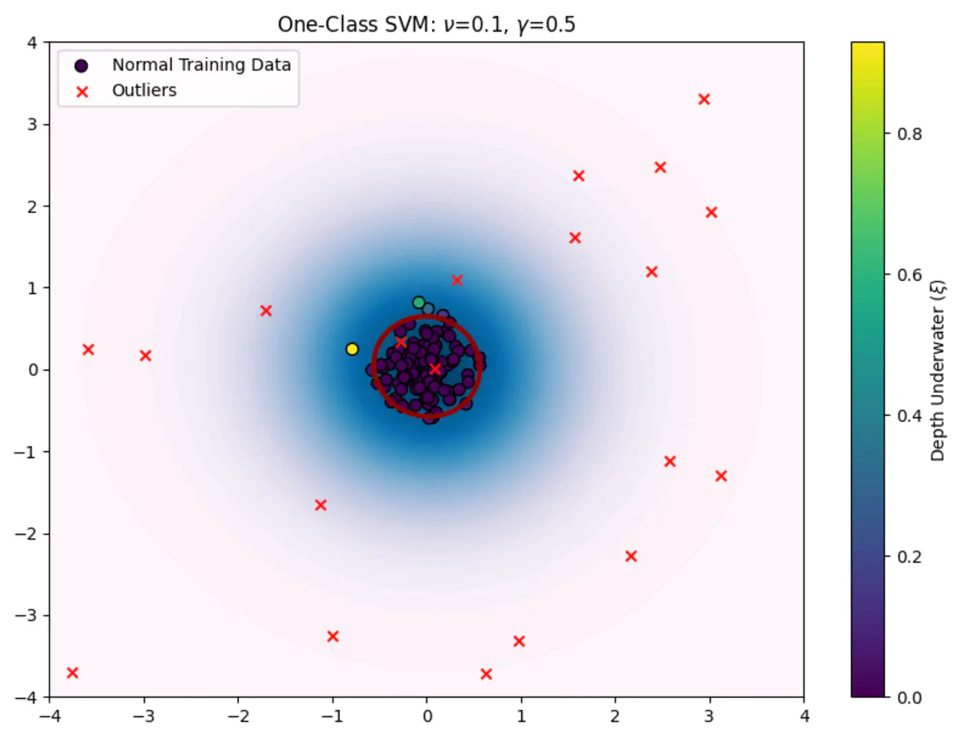
5.3 - One Class SVM
⭐️Only one class of data (normal, non-outlier) is available for training, making standard supervised learning models impossible.
e.g. Only normal observations are available for fraud detection, cyber attack, fault detection etc.

🦂 The core problem is to build a model that can distinguish between ‘normal’ and ‘anomalous’ data when we only have examples of the ‘normal’ class during training.
🦖 We need to find a decision boundary that is as compact as possible while still encompassing the bulk of the training data.
🦍 Define a boundary for a single class in high-dimensional space where data might be non-linearly distributed (e.g.‘U’ shape).
🦧 Use the Kernel Trick to project data into a higher-dimensional space and find a hyperplane that separates the data from the origin with the maximum margin.
⭐️OC-SVM, as introduced by Bernhard Schölkopf et al., uses a hyperplane ‘H’ defined by a weight vector \(\mathbf{w}\) and a bias term \(\rho\).
👉Solve the following optimization problem:
\[\min _{\mathbf{w},\xi _{i},\rho }\frac{1}{2}||\mathbf{w}||^{2}+\frac{1}{\nu N}\sum _{i=1}^{N}\xi _{i}-\rho \]Subject to constraints:
\[\mathbf{w}\cdot \phi (\mathbf{x}_{i})\ge \rho -\xi _{i}\quad \text{and}\quad \xi _{i}\ge 0,\quad \text{for\ }i=1,\dots ,N\]- \(\mathbf{x}_{i}\): i-th training data point.
- \(\phi (\mathbf{x}_{i})\): RBF kernel function \(K(x, y) = \exp(-\gamma \|x-y\|^2)\) that maps the data into a higher-dimensional feature space, making it easier to separate from the origin.
- \(\mathbf{w}\): normal vector to the separating hyperplane.
- \(\rho\): scalar bias term that determines the offset of the hyperplane from the origin.
- \(\xi_i\): Slack variables that allow some data points to fall on the ‘wrong’ side of the hyperplane (inside the anomalous region) to prevent overfitting.
- N: total number of training points.
- \(\nu\): hyper-parameter between 0 and 1. It acts as an upper bound on the fraction of outliers (training data points outside the boundary) and a lower bound on the fraction of support vectors.
- \(\frac{1}{2}\|\mathbf{w}\|^{2}\): aims to maximize the margin/compactness of the region.
- \(\frac{1}{\nu N}\sum _{i=1}^{N}\xi _{i}-\rho\): penalizes points (outliers) that violate the boundary constraints.
After solving the optimization problem using standard quadratic programming techniques, we obtain the optimal \(\mathbf{w}^{*}\) and \(\rho ^{*}\).
For a new data point \(x_{new}\), decision function is:
\[f(\mathbf{x}_{\text{new}})=\text{sign}(\mathbf{w}^{*}\cdot \phi (\mathbf{x}_{\text{new}})-\rho ^{*})\]\(f(\mathbf{x}_{\text{new}})\ge 0\): normal point.
\(f(\mathbf{x}_{\text{new}})< 0\): anomalous point (outlier).
End of Section
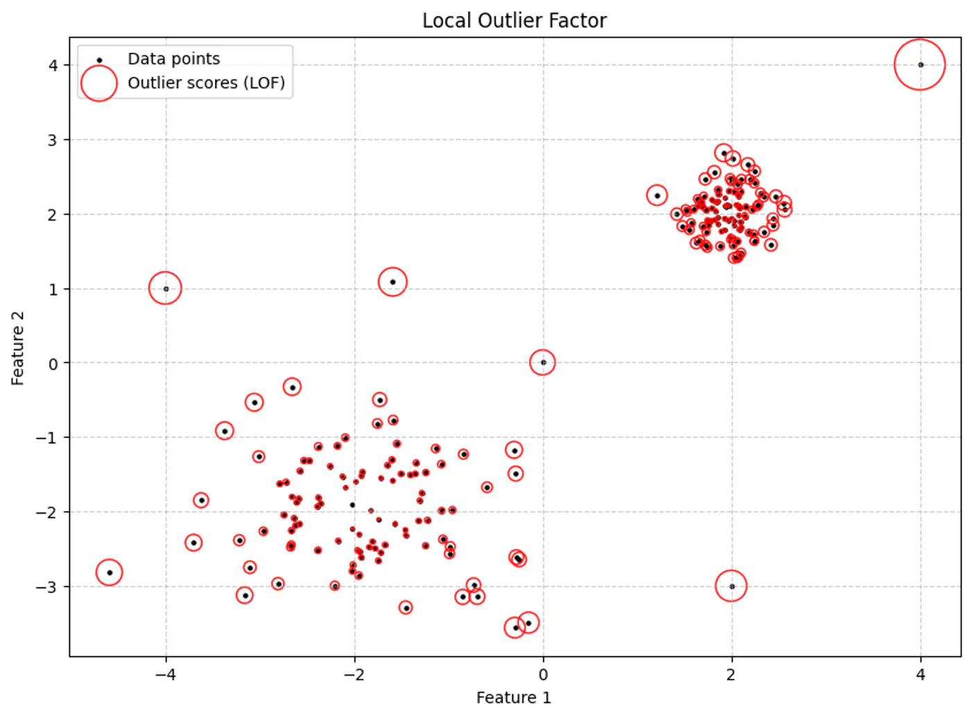
5.4 - Local Outlier Factor
A $100 transaction might be ‘normal’ in New York but an ‘outlier’ in a small rural village.
‘Local context matters.’
Global distance metrics fail when density is non-uniform.
🦄 An outlier is a point that is ‘unusual’ relative to its immediate neighbors, regardless of how far it is from the center of the entire dataset.
💡Traditional distance-based outlier detection methods, such as, KNN, often struggle with datasets where data is clustered at varying densities.
- A point in a sparse region might be considered an outlier by a global method, even if it is a normal part of that sparse cluster.
- Conversely, a point very close to a dense cluster might be an outlier relative to that specific neighborhood.
👉Calculate the relative density of a point compared to its immediate neighborhood.
e.g. If the neighbors are in a dense crowd and the point is not, it is an outlier.
Local Outlier Factor (LOF) is a density-based algorithm designed to detect anomalies by measuring the local deviation of a data point relative to its neighbors.
👉Size of the red circle represents the LOF score.
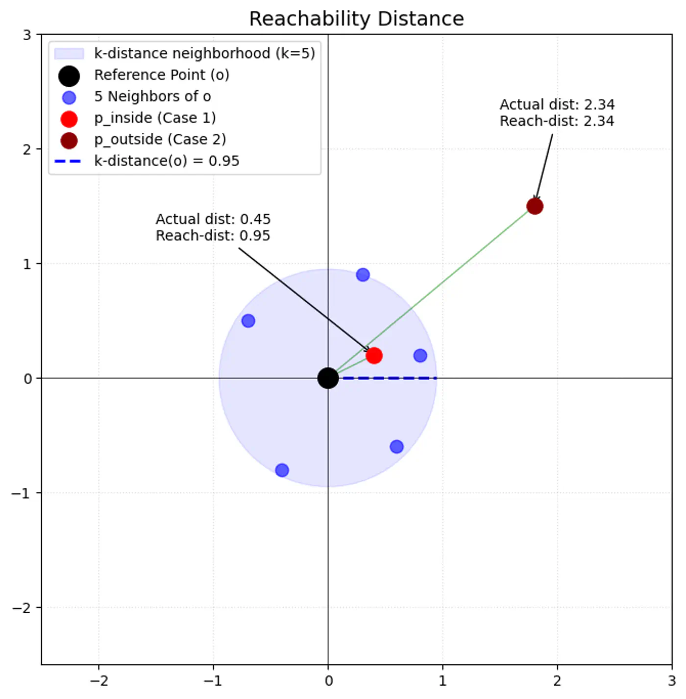
- K-Distance (\(k\text{-dist}(p)\)):
- The distance from point ‘p’ to its k-th nearest neighbor.
- Reachability Distance (\(\text{reach-dist}_{k}(p,o)\)):
\[\text{reach-dist}_{k}(p,o)=\max \{k\text{-dist}(o),\text{dist}(p,o)\}\]
- \(\text{dist}(p,o)\): actual Euclidean distance between ‘p’ and ‘o’.
- This acts as ‘smoothing’ factor.
- If point ‘p’ is very close to ‘o’ (inside o’s k-neighborhood), round up distance to \(k\text{-dist}(o)\).
- \(\text{dist}(p,o)\): actual Euclidean distance between ‘p’ and ‘o’.
- Local Reachability Density (\(\text{lrd}_{k}(p)\)):
- The inverse of the average reachability distance from ‘p’ to its k-neighbors (\(N_{k}(p)\)).
\[\text{lrd}_{k}(p)=\left[\frac{1}{|N_{k}(p)|}\sum _{o\in N_{k}(p)}\text{reach-dist}_{k}(p,o)\right]^{-1}\]
- High LRD: Neighbors are very close; the point is in a dense region.
- Low LRD: Neighbors are far away; the point is in a sparse region.
- The inverse of the average reachability distance from ‘p’ to its k-neighbors (\(N_{k}(p)\)).
\[\text{lrd}_{k}(p)=\left[\frac{1}{|N_{k}(p)|}\sum _{o\in N_{k}(p)}\text{reach-dist}_{k}(p,o)\right]^{-1}\]
- Local Outlier Factor (\(\text{LOF}_{k}(p)\)):
- The ratio of the average ‘lrd’ of p’s neighbors to p’s own ‘lrd’. \[\text{LOF}_{k}(p)=\frac{1}{|N_{k}(p)|}\sum _{o\in N_{k}(p)}\frac{\text{lrd}_{k}(o)}{\text{lrd}_{k}(p)}\]
- LOF ≈ 1: Point ‘p’ has similar density to its neighbors (inlier).
- LOF > 1: Point p’s density is much lower than its neighbors’ density (outlier).
End of Section
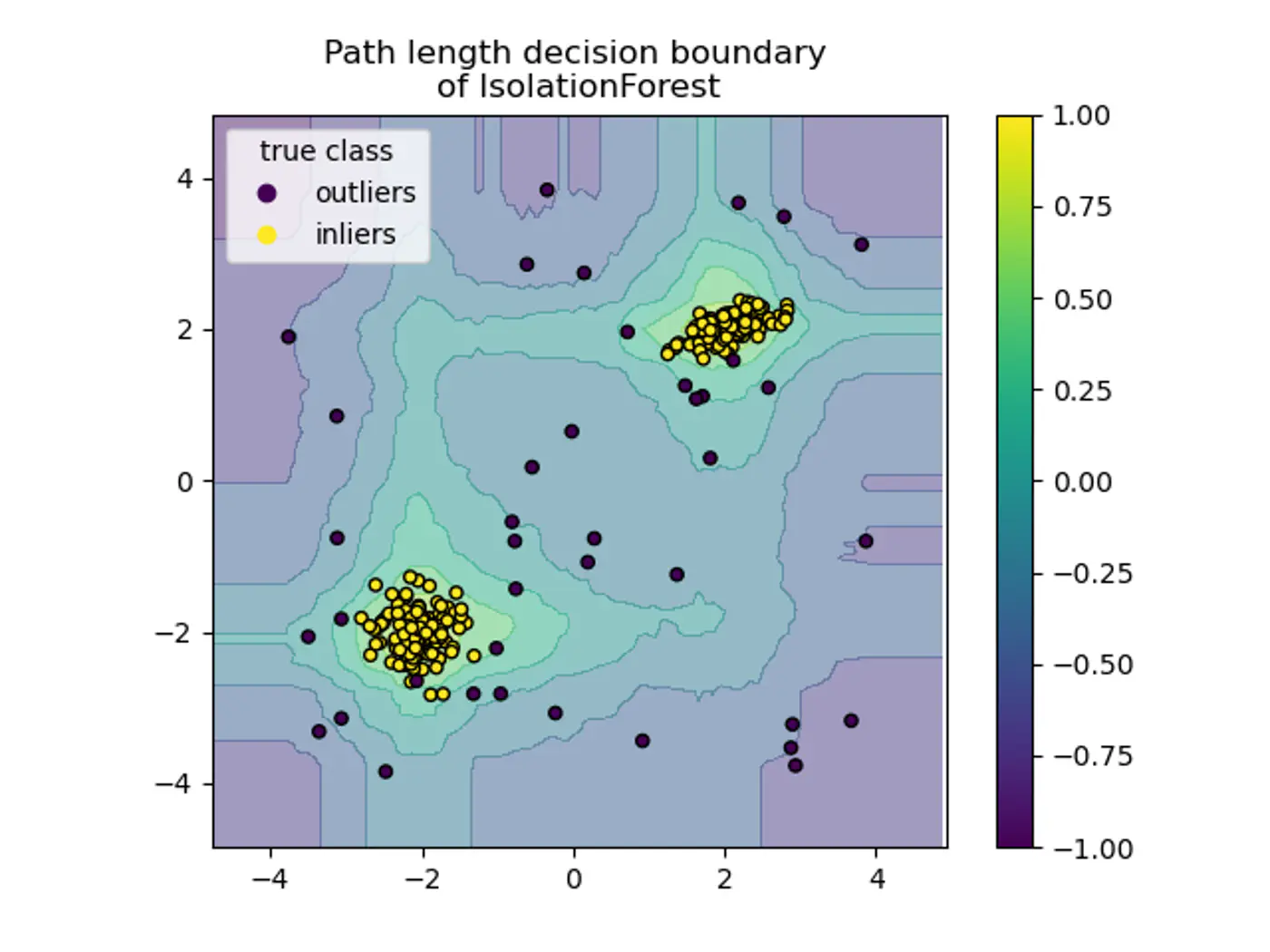
5.5 - Isolation Forest
‘Large scale tabular data.’
Credit card fraud detection in datasets with millions of rows and hundreds of features.
Note: Supervised learning requires balanced, labeled datasets (normal vs. anomaly), which are rarely available in real-world scenarios like fraud or cyber-attacks.
🦥 ‘Flip the logic.’
🦄 ‘Anomalies’ are few and different, so they are much easier to isolate from the rest of the data than normal points.
🐦🔥 ‘Curse of dimensionality.’
🐎 Distance based (K-NN), and density based (LOF) algorithms require calculation of distance between all pair of points.
🐙 As the number of dimensions and data points grows, these calculations become exponentially more expensive 💰 and less effective.
‘Randomly partition the data.’
🦄 If a point is an outlier, it will take fewer partitions (splits) to isolate it into a leaf 🍃 node compared to a point that is buried deep within a dense cluster of normal data.
🌳Isolation Forest uses an ensemble of ‘Isolation Trees’ (iTrees) 🌲.
👉iTree (Isolation Tree) 🌲 is a proper binary tree structure specifically designed to separate individual data points through random recursive partitioning.
- Sub-sampling:
- Select a random subset of data (typically 256 instances) to build an iTree.
- Tree Construction: Randomly select a feature.
- Randomly select a split value between the minimum and maximum values of that feature.
- Divide the data into two branches based on this split.
- Repeat recursively until the point is isolated or a height limit is reached.
- Forest Creation:
- Repeat 🔁 the process to create ‘N’ trees (typically 100).
- Inference:
- Pass a new data point through all trees, calculate the average path length, and compute the anomaly score.
⭐️🦄 Assign an anomaly score based on the path length h(x) required to isolate a point ‘x’.
- Path Length (h(x)): The number of edges ‘x’ traverses from the root node to a leaf node.
- Average Path Length (c(n)): Since iTrees are structurally similar to Binary Search Trees (BST), the average path length for a dataset of size ’n’ is given by: \[c(n)=2H(n-1)-\frac{2(n-1)}{n}\]
where, H(i) is the harmonic number, estimated as \(\ln (i)+0.5772156649\) (Euler’s constant).
To normalize the score between 0 and 1, we define it as:
\[s(x,n)=2^{-\frac{E(h(x))}{c(n)}}\]👉E(H(x)): is the average path length of across a forest of trees 🌲.
- \(s\rightarrow 1\): Point is an anomaly; Path length is very short.
- \(s\approx 0.5\): Point is normal, path length approximately equal to c(n).
- \(s\rightarrow 0\): Point is normal; deeply buried point, path length is much larger than c(n).
- Axis-Parallel Splits:
- Standard iTrees 🌲 split only on one feature at a time, so:
- We do not get a smooth decision boundary.
- Anything off-axis has a higher probability of being marked as an outlier.
- Note: Extended Isolation Forest fixes this by using random slopes.
- Standard iTrees 🌲 split only on one feature at a time, so:
- Score Sensitivity: The threshold for what constitutes an ‘anomaly’ often requires manual tuning or domain knowledge.
End of Section
5.6 - RANSAC
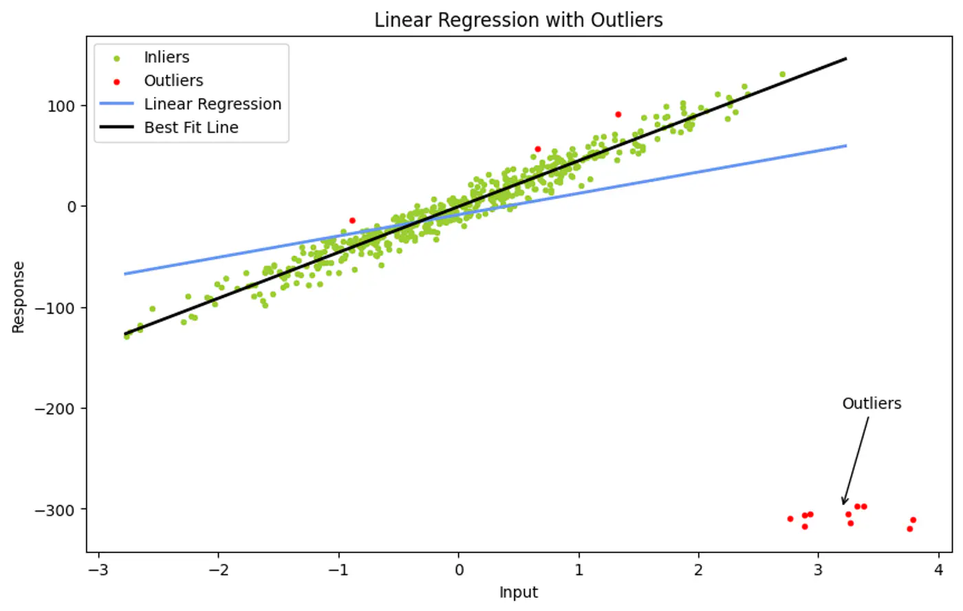
👉Ordinary Least Squares use all data points to find a fit.
- However, a single outlier can ‘pull’ the resulting line significantly, leading to a poor representative model.
💡If we pick a very small random subset of points, there is a higher probability that this small subset contains only good data (inliers) compared to a large set.
Ordinary Least Squares (OLS) minimizes the Sum of Errors.
- A huge outlier has an exponentially large impact on the final line.
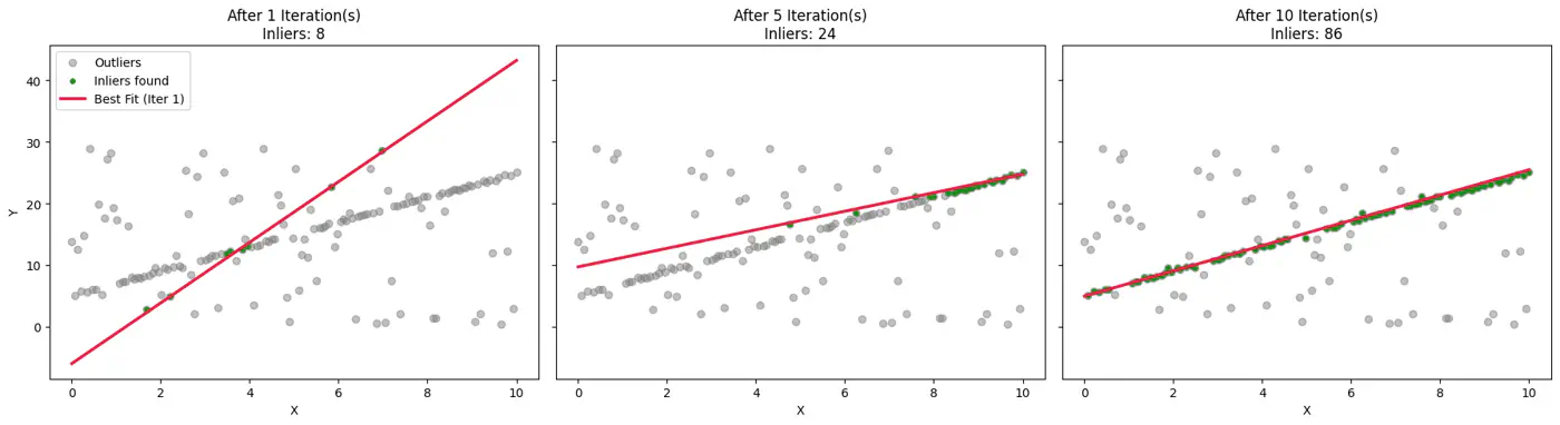
💡Instead of using all points, iteratively pick the smallest possible random subset to fit a model, then check (votes) how many other points in the dataset ‘agree’ with that model.
This gives the name to our algorithm:
- Random: Random subsets.
- Sampling: Small subsets.
- Consensus: Agreement with other points.
- Random Sampling:
- Randomly select a Minimal Sample Set (MSS) of ’n’ points from the input data ‘D’.
- e.g. n=2 for a line, or n=3 for a plane in 3D.
- Model Fitting:
- Compute the model parameters using only these ’n’ points.
- Test:
- For all other points in ‘D’, calculate the error relative to the model.
- 👉 Points with error < \(\tau\)(threshold) are added to the ‘Consensus Set’.
- Evaluate:
- If the consensus set is larger than the previous best, save this model and set.
- Repeat 🔁:
- Iterate ‘k’ times.
- Refine (Optional):
- Once the best model is found, re-estimate it using all points in the final consensus set (usually via Least Squares) for a more precise fit.
👉Example:
👉To ensure the algorithm finds a ‘clean’ sample set (no outliers) with a desired probability(often 99%), we use the following formula:
\[k=\frac{\log (1-P)}{\log (1-w^{n})}\]- k: Number of iterations required.
- P: Probability that at least one random sample contains only inliers.
- w: Ratio of inliers in the dataset (number of inliers / total points).
- n: Number of points in the Minimal Sample Set.
End of Section
6 - Dimensionality Reduction
6.1 - PCA
- Data Compression
- Noise Reduction
- Feature Extraction: Create a smaller set of meaningful features from a larger one.
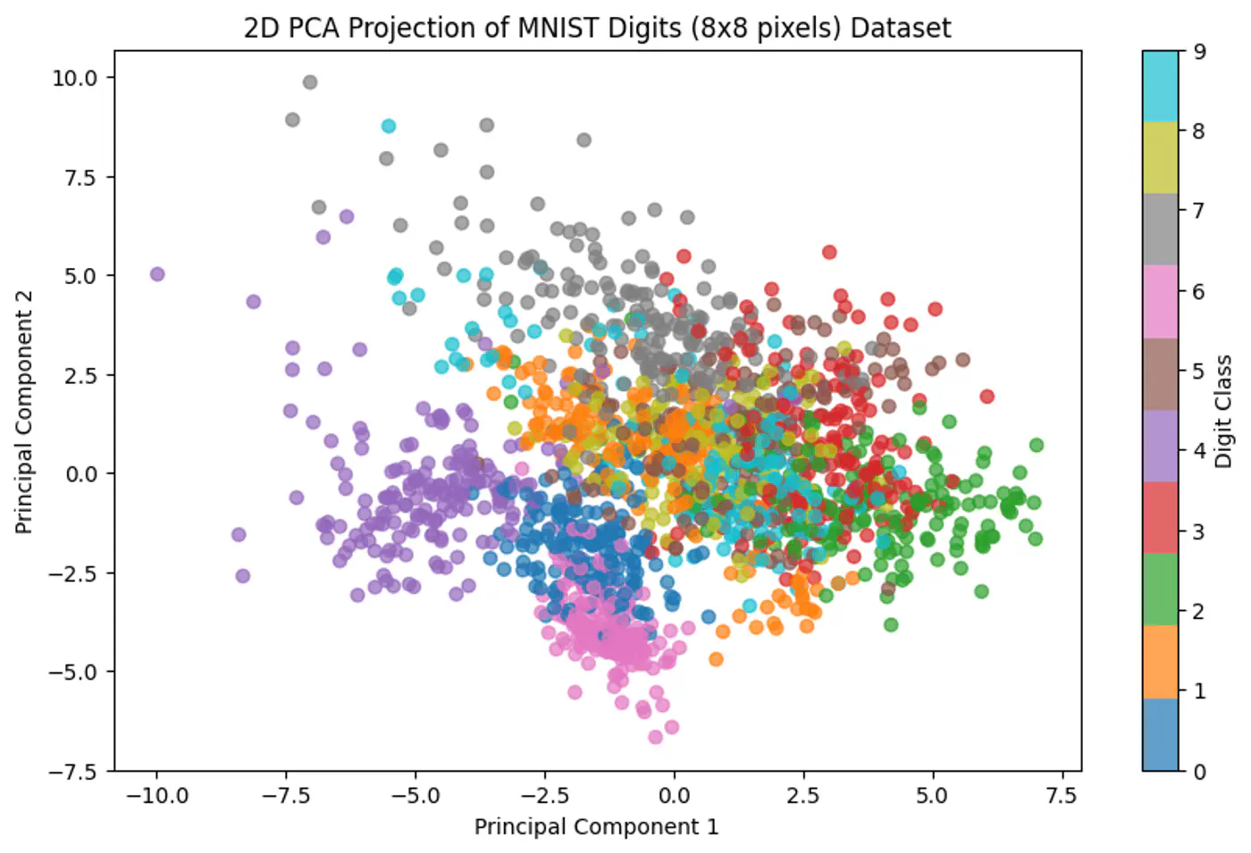
- Data Visualization: Project high-dimensional data down to 2 or 3 dimensions.
Assumption: Linear relationship between features.
💡‘Information = Variance’
☁️ Imagine a cloud of points in 2D space.
👀 Look for the direction (axis) along which the data is most ‘spread out’.
🚀 By projecting data onto this axis, we retain the maximum amount of information (variance).
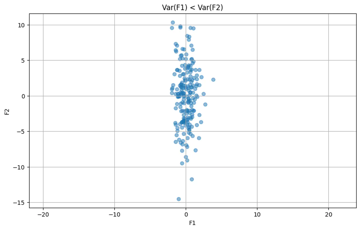
👉Example 1: Var(Feature 1) < Var(Feature 1)
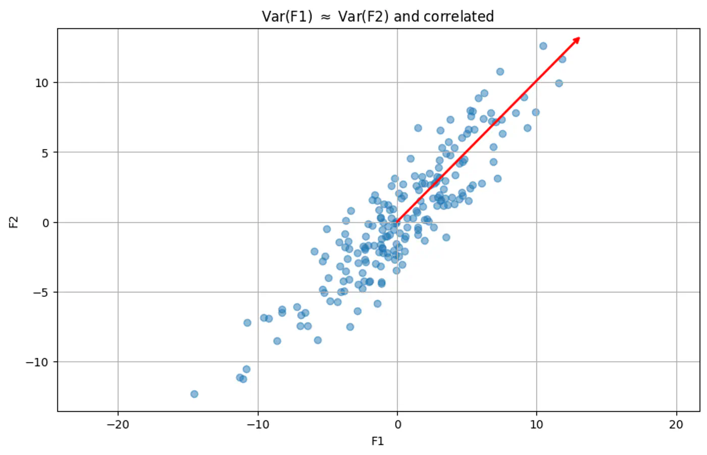
👉Example 2: Red line shows the direction of maximum variance
🧭 Finds the direction of maximum variance in the data.
Note: Some loss of information will always be there in dimensionality reduction, because there will be some variability in data along the direction that is dropped, and that will be lost.
- PCA seeks a direction 🧭, represented by a unit vector \(\hat{u}\) onto which data can be projected to maximize variance.
- The projection of a mean centered data point \(x_i\) onto \(u\) is \(u^Tx_i\).
- The variance of these projections can be expressed as \(u^{T}\Sigma u\), where \(\Sigma\) is the data’s covariance matrix.
- Data: Let \(X = \{x_{1},x_{2},\dots ,x_{n}\}\) is the mean centered (\(\bar{x} = 0\)) dataset.
- Projection of point \(x_i\) on \(u\) is \(z_i = u^Tx_i\)
- Variance of projected points (since \(\bar{x} = 0\)): \[\text{Var}(z)=\frac{1}{n}\sum _{i=1}^{n}z_{i}^{2}=\frac{1}{n}\sum _{i=1}^{n}(x_{i}^{T}u)^{2}\]
- 💡Since, \((x_{i}^{T}u)^{2} = (u^{T}x_{i})(x_{i}^{T}u)\) \( \implies\text{Var}(z)=u^{T}\left(\frac{1}{n}\sum _{i=1}^{n}x_{i}x_{i}^{T}\right)u\)
- 💡Since, Covariance Matrix, \(\Sigma = \left(\frac{1}{n}\sum _{i=1}^{n}x_{i}x_{i}^{T}\right)\)
- 👉 Therefore, \(\text{Var}(z)=u^{T}\Sigma u\)
👉 To prevent infinite variance, PCA constrains \(u\) to be a unit vector (\(\|u\|=1\)).
\[\text{maximize\ }u^{T}\Sigma u, \quad \text{subject\ to\ }u^{T}u=1\]Note: This constraint forces the optimization algorithm to focus purely on the direction that maximizes variance, rather than allowing it to artificially inflate the variance by increasing the length of the vector.
⏲️ Lagrangian function: \(L(u,\lambda )=u^{T}\Sigma u-\lambda (u^{T}u-1)\)
🔦 To find \(u\) that maximizes above constrained optimization:
💎 This is the standard Eigenvalue Equation.
🧭 So, the optimal directions \(u\) are the eigenvectors of the covariance matrix \(\Sigma\).
👉 To see which eigenvector maximizes variance, substitute the result back into the variance equation:
\[\text{Variance}=u^{T}\Sigma u=u^{T}(\lambda u)=\lambda (u^{T}u)=\lambda \]🧭 Since the variance equals the eigenvalue \(\lambda\), the direction \(u\) that maximizes variance is the eigenvector associated with the largest eigenvalue.
- Center the data: \(X = X - \mu\)
- Compute the Covariance Matrix: \(\Sigma = \frac{1}{n-1} X^T X\)
- Compute Eigenvectors and Eigenvalues of \(\Sigma\) .
- Sort eigenvalues in descending order and select the top ‘k’ eigenvectors.
- Project the original data onto the subspace: \(Z = X W_k\) where, \(W_{k}=[u_{1},u_{2},\dots ,u_{k}]\) , matrix formed by ‘k’ eigenvectors corresponding to ‘k’ largest eigenvalues.
- Cannot model non-linear relationships.
- Sensitive to outliers.
End of Section
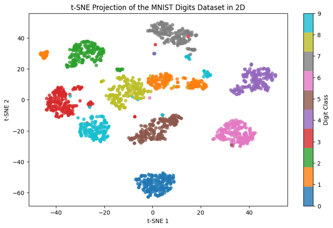
6.2 - t-SNE
👉 PCA preserves variance, not neighborhoods.
🔬 t-SNE focuses on the ‘neighborhood’ (local structure).
💡Tries to keep points that are close together in high-dimensional space close together in low-dimensional space.
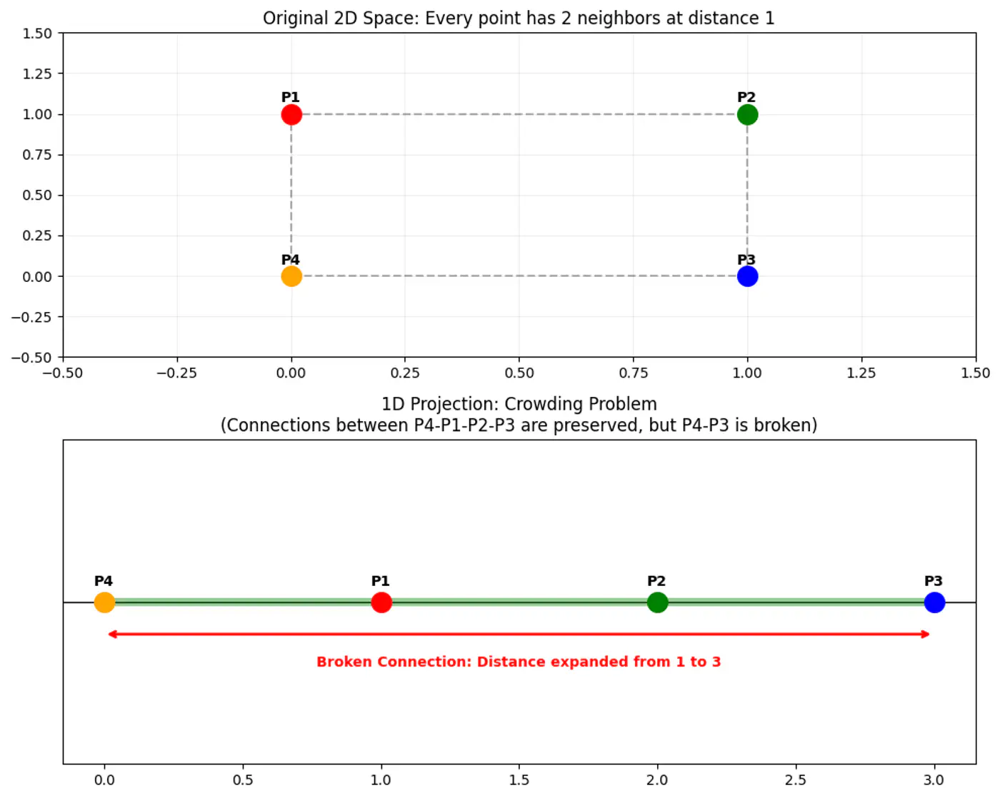
👉 Map high-dimensional points to low-dimensional points , such that the pairwise similarities are preserved, while solving the ‘crowding problem’ (where points collapse into a single cluster).
👉 Crowding Problem
📌 Convert Euclidean distances into conditional probabilities representing similarities.
⚖️ Minimize the divergence between the probability distributions of the high-dimensional (Gaussian)
and low-dimensional (t-distribution) spaces.
Note: Probabilistic approach to defining neighbors is the core ‘stochastic’ element of the algorithm’s name.
💡The similarity of datapoint \(x_j\) to datapoint \(x_i\) is the conditional probability \(p_{j|i}\), that \(x_i\) would pick \(x_j\) as its neighbor.
Note: If neighbors are picked in proportion to their probability density under a Gaussian centered at \(x_i\).
\[p_{j|i} = \frac{\exp(-||x_i - x_j||^2 / 2\sigma_i^2)}{\sum_{k \neq i} \exp(-||x_i - x_k||^2 / 2\sigma_i^2)}\]- \(p_{j|i}\) high: nearby points.
- \(p_{j|i}\) low: widely separated points.
Note: Make probabilities symmetric: \(p_{ij} = \frac{p_{j|i} + p_{i|j}}{2n}\)
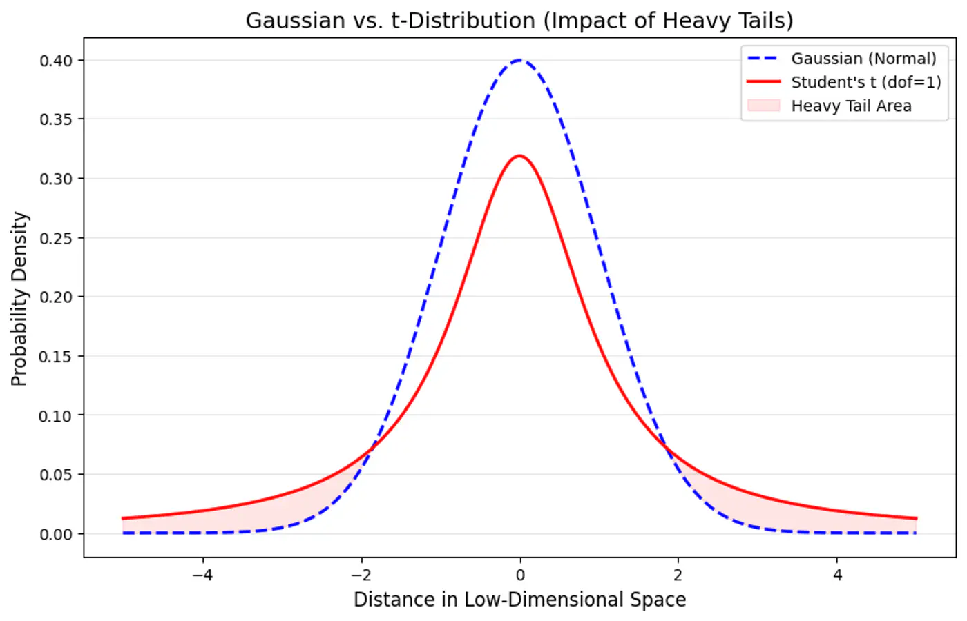
🧠 To solve the crowding problem, we use a heavy-tailed 🦨 distribution (Student’s-t distribution with degree of freedom \(\nu=1\)).
\[q_{ij} = \frac{(1 + ||y_i - y_j||^2)^{-1}}{\sum_{k \neq l} (1 + ||y_k - y_l||^2)^{-1}}\]Note: Heavier tail spreads out dissimilar points more effectively, allowing moderately distant points to be mapped further apart, preventing clusters from collapsing and ensuring visual separation and cluster distinctness.
👉 Measure the difference between the distributions ‘p’ and ‘q’ using the Kullback-Leibler (KL) divergence, which we aim to minimize:
\[C = KL(P||Q) = \sum_i \sum_j p_{ij} \log \frac{p_{ij}}{q_{ij}}\]🏔️ Use gradient descent to iteratively adjust the positions of the low-dimensional points \(y_i\).
👉 The gradient of the KL divergence is:
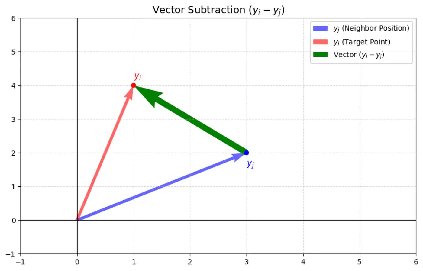
\[\frac{\partial C}{\partial y_{i}}=4\sum _{j\ne i}(p_{ij}-q_{ij})(y_{i}-y_{j})(1+||y_{i}-y_{j}||^{2})^{-1}\]- C : t-SNE cost function (sum of all KL divergences).
- \(y_i, y_j\): coordinates of data points and in the low-dimensional space (typically 2D or 3D).
- \(p_{ij}\): high-dimensional similarity (joint probability) between points \(x_i\) and \(x_j\), calculated using a Gaussian distribution.
- \(q_{ij}\): low-dimensional similarity (joint probability) between points \(y_i\) and \(y_j\), calculated using a Student’s t-distribution with one degree of freedom.
- \((1+||y_{i}-y_{j}||^{2})^{-1}\): term comes from the heavy-tailed Student’s t-distribution, which helps mitigate the ‘crowding problem’ by allowing points that are moderately far apart to have a small attractive force.
💡 The gradient can be understood as a force acting on each point \(y_i\) in the low-dimensional map:
\[\frac{\partial C}{\partial y_{i}}=4\sum _{j\ne i}(p_{ij}-q_{ij})(y_{i}-y_{j})(1+||y_{i}-y_{j}||^{2})^{-1}\]- Attractive forces: If \(p_{ij}\) is large ⬆️ and \(q_{ij}\) is small ⬇️ (meaning two points were close in the high-dimensional space but are far in the low-dimensional space), the term \((p_{ij}-q_{ij})\) is positive, resulting in a strong attractive force pulling \(y_i\) and \(y_j\) closer.
- Repulsive forces: If \(p_{ij}\) is small ⬇️ and \(q_{ij}\) is large ⬆️ (meaning two points were far in the high-dimensional space but are close in the low-dimensional space), the term \((p_{ij}-q_{ij})\) is negative, resulting in a repulsive force pushing \(y_i\) and \(y_j\) apart.
👉 Update step of in low dimensions:
\[y_{i}^{(t+1)}=y_{i}^{(t)}-\eta \frac{\partial C}{\partial y_{i}}\]Attractive forces (\(p_{ij}>q_{ij}\)):
- The negative gradient moves \(y_i\) opposite to the (\(y_i - y_j\)) vector, pulling it toward \(y_j\).
Repulsive forces (\(p_{ij} < q_{ij}\)):
- The negative gradient moves \(y_i\) in the same direction as the (\(y_i - y_j\)) vector, pushing it away from \(y_j\).
🏘️ User-defined parameter that loosely relates to the effective number of neighbors.
Note: Variance \(\sigma_i^2\) (Gaussian) is adjusted for each point to maintain a consistent perplexity.
End of Section
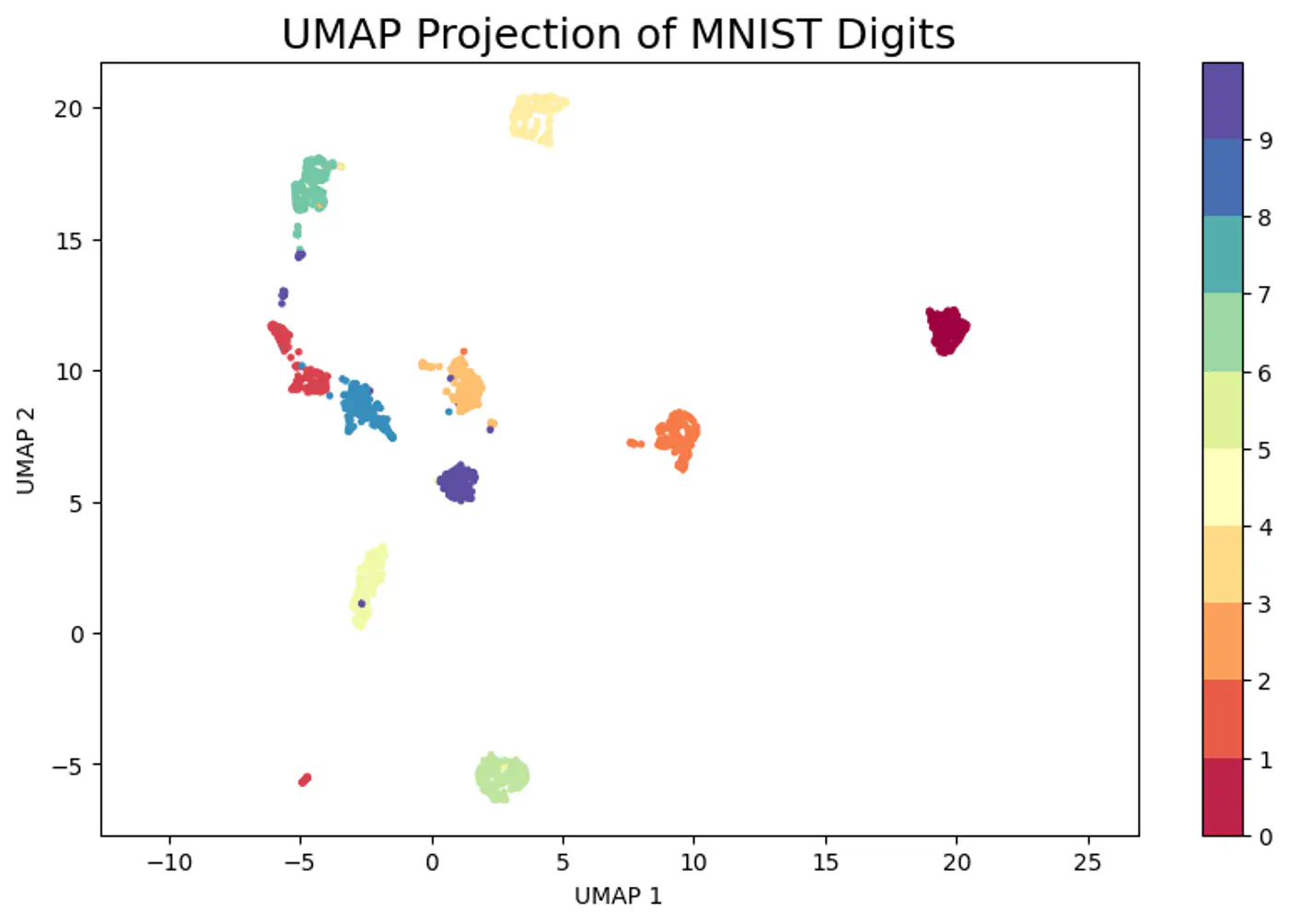
6.3 - UMAP
🐢Visualizing massive datasets where t-SNE is too slow.
⭐️ Creating robust low-dimensional inputs for subsequent machine learning models.
⭐️ Using a world map 🗺️ (2D)instead of globe 🌍 for spherical(3D) earth 🌏.
👉It preserves the neighborhood relationships of countries (e.g., India is next to China), and to a good degree, the global structure.
⭐️ Non-linear dimensionality reduction technique to visualize high-dimensional data (like images, gene expressions)
in a lower-dimensional space (typically 2D or 3D), preserving its underlying structure and relationships.
👉 Constructs a high-dimensional graph of data points and then optimizes a lower-dimensional layout to closely match this graph, making complex datasets understandable by revealing patterns, clusters, and anomalies.
Note: Similar to t-SNE but often faster and better at maintaining global structure.
💡 Create a weighted graph (fuzzy simplicial set) representing the data’s topology and then find a low-dimensional graph that is as structurally similar as possible.
Note: Fuzzy means instead of using binary 0/1, we use weights in the range [0,1] for each edge.
- UMAP determines local connectivity based on a user-defined number of neighbors (n_neighbors).
- Normalizes distances locally using the distance to the nearest neighbor (\(\rho_i\)) and a scaling factor (\(\sigma_i\)) adjusted to enforce local connectivity constraints.
- The weight \(W_{ij}\) (fuzzy similarity) in high-dimensional space is: \[W_{ij}=\exp \left(-\frac{\max (0,\|x_{i}-x_{j}\|-\rho _{i})}{\sigma _{i}}\right)\]
Note: This ensures that the closest point always gets a weight of 1, preserving local structure.
👉In the low-dimensional space (e.g., 2D), UMAP uses a simple curve (similar to the t-distribution used in t-SNE) for edge weights:
\[Z_{ij}=(1+a\|y_{i}-y_{j}\|^{2b})^{-1}\]Note: The parameters ‘a’ and ‘b’ are typically fixed based on the ‘min_dist’ user parameter (e.g. min_dist = 0.1, then a≈1,577, b≈0.895).
⭐️ Unlike t-SNE’s KL divergence, UMAP minimizes the cross-entropy between the high-dimensional weights \(W_{ij}\) and the low-dimensional weights \(Z_{ij}\).
👉 Cost 💰 Function (C):
\[C=\sum _{i,j}\left(W_{ij}\log \frac{W_{ij}}{Z_{ij}}+(1-W_{ij})\log \frac{1-W_{ij}}{1-Z_{ij}}\right)\]Cost 💰 Function (C):
\[C=\sum _{i,j}\left(W_{ij}\log \frac{W_{ij}}{Z_{ij}}+(1-W_{ij})\log \frac{1-W_{ij}}{1-Z_{ij}}\right)\]🎯 Goal : Reduce overall Cross Entropy Loss.
- Attractive Force: \(W_{ij}\) high; make \(Z_{ij}\) high to make the log \(\frac{W_{ij}}{Z_{ij}} \)term small.
- Repulsive Force: \(W_{ij}\) low; make \(Z_{ij}\) low to make the \(log\frac{1-W_{ij}}{1-Z_{ij}}\) term small.
Note: This push and pull of 2 ‘forces’ will make the data in low dimensions settle into a position that is overall a good representation of the original data in higher dimensions.
- Mathematically complex.
- Requires tuning (n_neighbors, min_dist).
End of Section