🦄 Anomaly is a rare item, event or observation which deviates significantly from the majority of the data and does not conform to a well-defined notion of normal behavior.

Note: Such examples may arouse suspicions of being generated by a different mechanism, or appear inconsistent with the remainder of that set of data.

❌ Remove Outliers:

• Rejection or omission of outliers from the data to aid statistical analysis, for example to compute the mean or standard deviation of the dataset.
• Remove outliers for better predictions from models, such as linear regression.

🔦Focus on Outliers:

• Fraud detection in banking and financial services.
• Cyber-security: intrusion detection, malware, or unusual user access patterns.

• Supervised
• Semi-Supervised
• Unsupervised (most common) ✅

Note: Labeled anomaly data is often unavailable in real-world scenarios.

• Statistical Methods: Z-Score, large value means outlier, IQR, point beyond fences (Q1 - 1.5*IQR or Q3 + 1.5*IQR) is flagged as an outlier.
• Distance Based: KNN, points far from their neighbors as potential anomalies.
• Density Based: DBSCAN, points in low density regions are considered outliers.
• Clustering Based: K-Means, points far from cluster centroids that do not fit any cluster are anomalies.

• Elliptic Envelope (MCD - Minimum Covariance Determinant)
• One-Class SVM (OC-SVM)
• Local Outlier Factor (LOF)
• Isolation Forest (iForest)
• RANSAC (Random Sample Consensus)

Detect anomalies in multivariate Gaussian data, such as, biometric data (height/weight) where features are normally distributed and correlated.

Assumption: The data can be modeled by a Gaussian distribution.

In a normal distribution, most data points cluster around the mean, and the probability density decreases as we move farther away from the center.

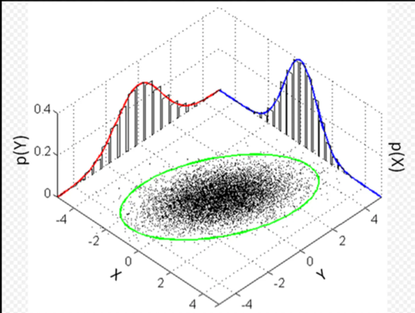
🌍 Euclidean distance measures the simple straight-line distance from the center of the cloud.

👉If the data is spherical, this works fine.

🦕 However, real-world data is often stretched or skewed (e.g., taller people are generally heavier), due to correlations between variables, forming an elliptical shape.

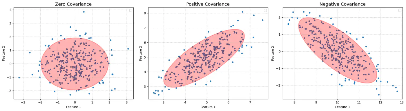
⭐️Mahalanobis distance essentially re-scales the data so that the elliptical distribution appears spherical, and then measures the Euclidean distance in that transformed space.

👉This way, it measures how many standard deviations(\(\sigma\)) away a point is from the mean, considering the data’s spread and correlation (covariance).

👉Find the most dense core of the data.

🦣 Determinant of covariance matrix \(\Sigma\) represents the volume of the ellipsoid.

⏲️ Therefore, minimize \(|\Sigma|\) to find the tight core.

👉 \(\text {Small} ~ \Sigma \rightarrow \text {Large} ~\Sigma ^{-1}\rightarrow \text {Large} ~ D_{M} ~\text {for outliers}\)

MCD algorithm is used to find the covariance matrix \(\Sigma\) with minimum determinant, so that the volume of the ellipsoid is minimized.

1. Initialization: Select several random subsets of size h < n (default h = \(\frac{n+d+1}{2}\), d = # dimensions), representing ‘robust’ majority of the data.
2. Calculate preliminary mean (\(\mu\)) and covariance (\(\Sigma\)) for each random subset.
3. Concentration Step: Iterative core of the algorithm designed to ‘tighten’ the ellipsoid.
   • Calculate Distances: Compute the Mahalanobis distance of all ’n’ points in the dataset from the current subset’s mean (\(\mu\)) and covariance (\(\Sigma\)).
   • Select New Subset: Identify the ‘h’ points with the smallest Mahalanobis distances.
     • These are the points most centrally located relative to the current ellipsoid.
   • Update Estimates: Calculate a new and based only on these ‘h’ most central points.
   • Repeat 🔁: The steps repeat until the determinant stops shrinking.

Note: Select the best subset that achieved the absolute minimum determinant.

• Assumptions
  • Gaussian data.
  • Unimodal data (single center).
• Cost 💰of covariance matrix \(\Sigma^{-1}\) inversion is O(d^3).

⭐️Only one class of data (normal, non-outlier) is available for training, making standard supervised learning models impossible.

e.g. Only normal observations are available for fraud detection, cyber attack, fault detection etc.

🦂 The core problem is to build a model that can distinguish between ‘normal’ and ‘anomalous’ data when we only have examples of the ‘normal’ class during training.

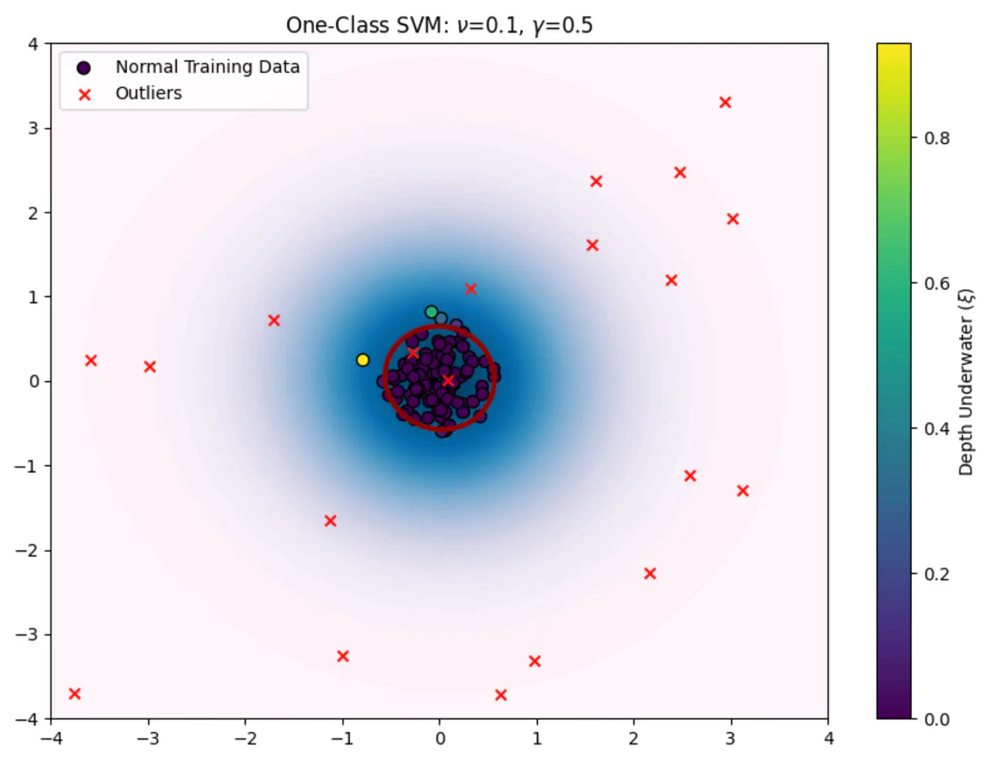
🦖 We need to find a decision boundary that is as compact as possible while still encompassing the bulk of the training data.

🦍 Define a boundary for a single class in high-dimensional space where data might be non-linearly distributed (e.g.‘U’ shape).

🦧 Use the Kernel Trick to project data into a higher-dimensional space and find a hyperplane that separates the data from the origin with the maximum margin.

⭐️OC-SVM, as introduced by Bernhard Schölkopf et al., uses a hyperplane ‘H’ defined by a weight vector \(\mathbf{w}\) and a bias term \(\rho\).

👉Solve the following optimization problem:

Subject to constraints:

• \(\mathbf{x}_{i}\): i-th training data point.
• \(\phi (\mathbf{x}_{i})\): RBF kernel function \(K(x, y) = \exp(-\gamma \|x-y\|^2)\) that maps the data into a higher-dimensional feature space, making it easier to separate from the origin.
• \(\mathbf{w}\): normal vector to the separating hyperplane.
• \(\rho\): scalar bias term that determines the offset of the hyperplane from the origin.
• \(\xi_i\): Slack variables that allow some data points to fall on the ‘wrong’ side of the hyperplane (inside the anomalous region) to prevent overfitting.
• N: total number of training points.
• \(\nu\): hyper-parameter between 0 and 1. It acts as an upper bound on the fraction of outliers (training data points outside the boundary) and a lower bound on the fraction of support vectors.

• \(\frac{1}{2}\|\mathbf{w}\|^{2}\): aims to maximize the margin/compactness of the region.
• \(\frac{1}{\nu N}\sum _{i=1}^{N}\xi _{i}-\rho\): penalizes points (outliers) that violate the boundary constraints.

After solving the optimization problem using standard quadratic programming techniques, we obtain the optimal \(\mathbf{w}^{*}\) and \(\rho ^{*}\).

For a new data point \(x_{new}\), decision function is:

• \(f(\mathbf{x}_{\text{new}})\ge 0\): normal point.

• \(f(\mathbf{x}_{\text{new}})< 0\): anomalous point (outlier).

  

‘Local context matters.’

Global distance metrics fail when density is non-uniform.

🦄 An outlier is a point that is ‘unusual’ relative to its immediate neighbors, regardless of how far it is from the center of the entire dataset.

💡Traditional distance-based outlier detection methods, such as, KNN, often struggle with datasets where data is clustered at varying densities.

• A point in a sparse region might be considered an outlier by a global method, even if it is a normal part of that sparse cluster.
• Conversely, a point very close to a dense cluster might be an outlier relative to that specific neighborhood.

👉Calculate the relative density of a point compared to its immediate neighborhood.

e.g. If the neighbors are in a dense crowd and the point is not, it is an outlier.

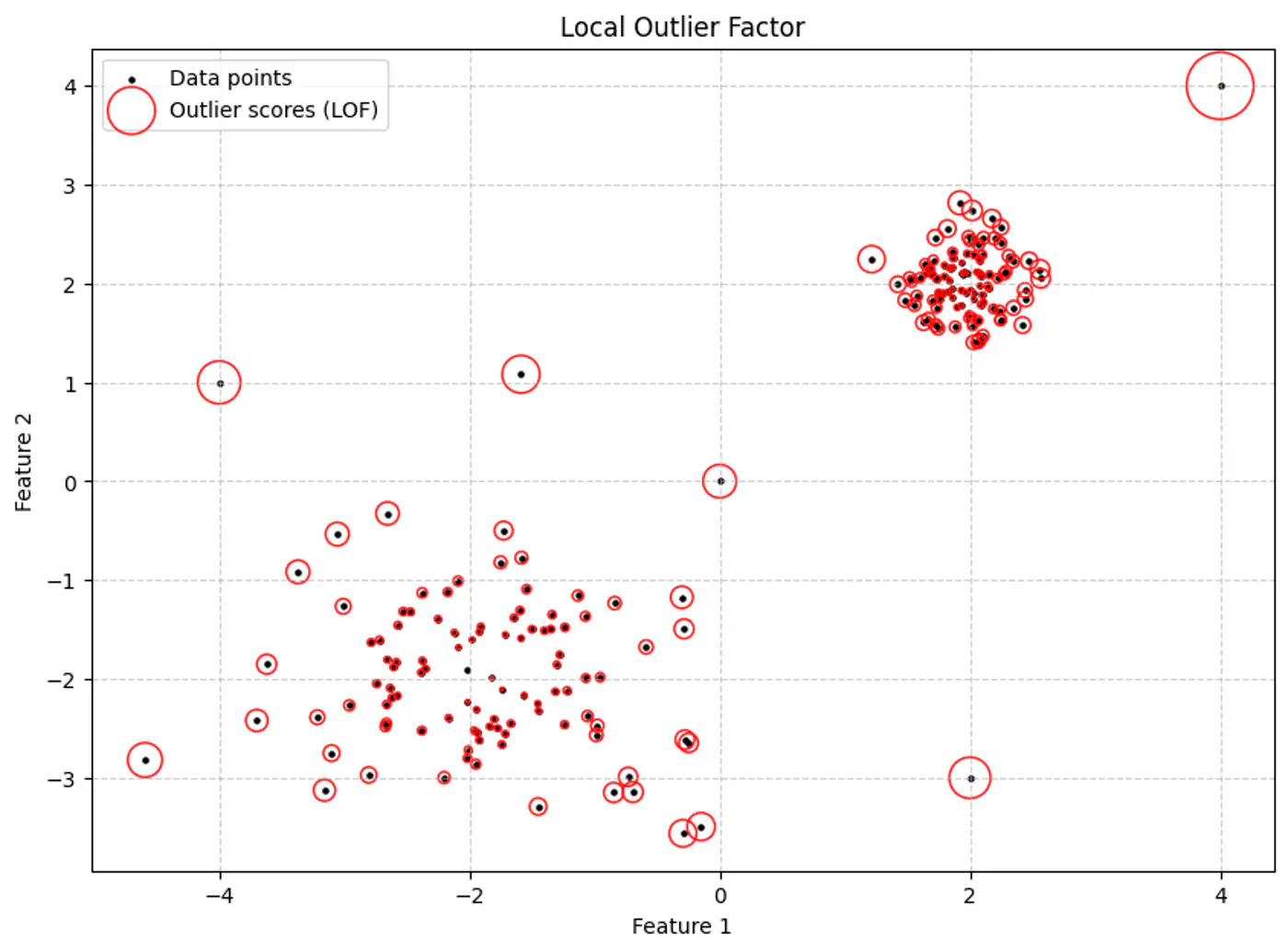
Local Outlier Factor (LOF) is a density-based algorithm designed to detect anomalies by measuring the local deviation of a data point relative to its neighbors.

👉Size of the red circle represents the LOF score.

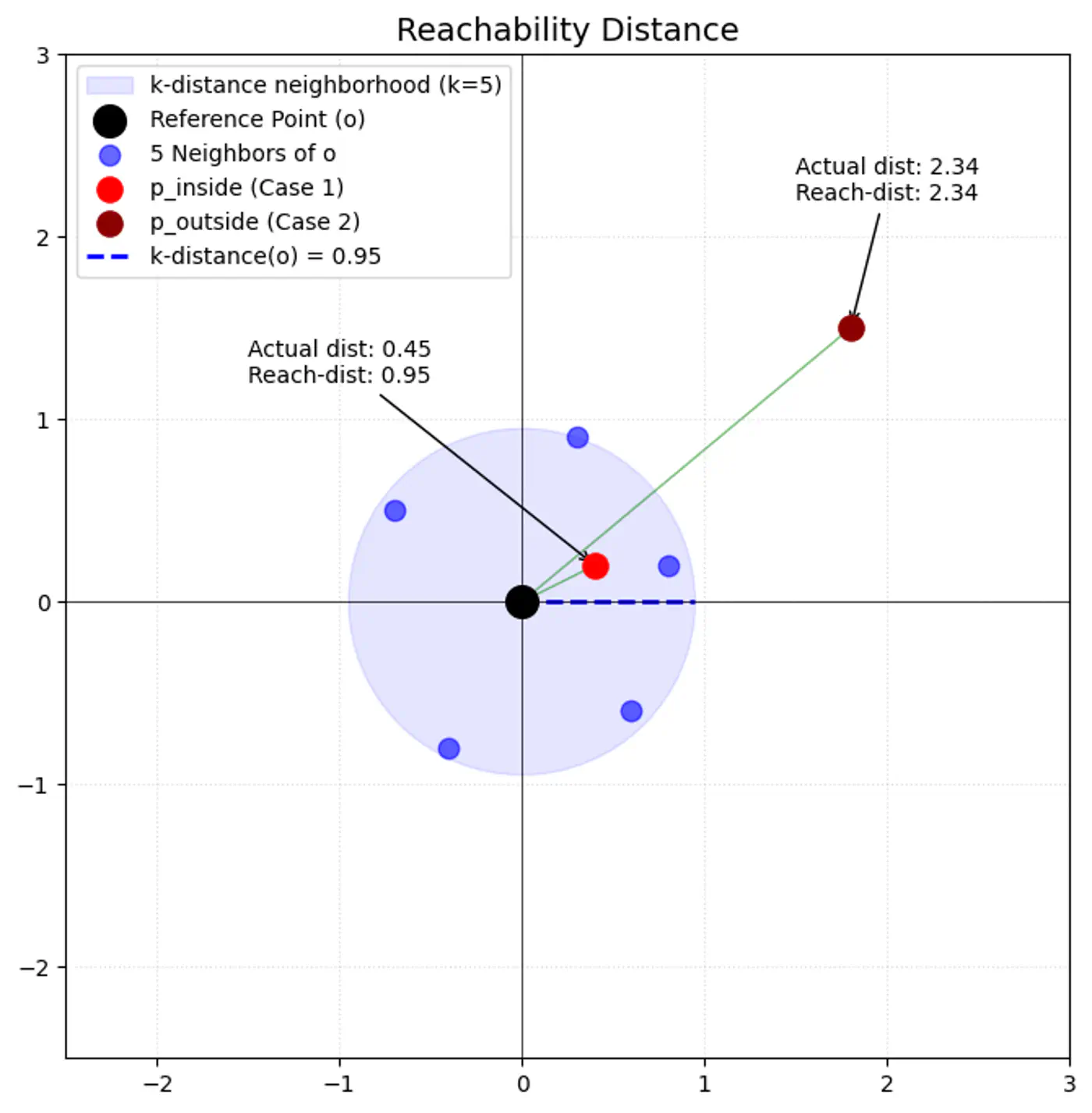
1. K-Distance (\(k\text{-dist}(p)\)):
   • The distance from point ‘p’ to its k-th nearest neighbor.
2. Reachability Distance (\(\text{reach-dist}_{k}(p,o)\)): \[\text{reach-dist}_{k}(p,o)=\max \{k\text{-dist}(o),\text{dist}(p,o)\}\]
   • \(\text{dist}(p,o)\): actual Euclidean distance between ‘p’ and ‘o’.
     
   • This acts as ‘smoothing’ factor.
   • If point ‘p’ is very close to ‘o’ (inside o’s k-neighborhood), round up distance to \(k\text{-dist}(o)\).
3. Local Reachability Density (\(\text{lrd}_{k}(p)\)):
   • The inverse of the average reachability distance from ‘p’ to its k-neighbors (\(N_{k}(p)\)). \[\text{lrd}_{k}(p)=\left[\frac{1}{|N_{k}(p)|}\sum _{o\in N_{k}(p)}\text{reach-dist}_{k}(p,o)\right]^{-1}\]
     • High LRD: Neighbors are very close; the point is in a dense region.
     • Low LRD: Neighbors are far away; the point is in a sparse region.
4. Local Outlier Factor (\(\text{LOF}_{k}(p)\)):
   • The ratio of the average ‘lrd’ of p’s neighbors to p’s own ‘lrd’. \[\text{LOF}_{k}(p)=\frac{1}{|N_{k}(p)|}\sum _{o\in N_{k}(p)}\frac{\text{lrd}_{k}(o)}{\text{lrd}_{k}(p)}\]

• LOF ≈ 1: Point ‘p’ has similar density to its neighbors (inlier).
• LOF > 1: Point p’s density is much lower than its neighbors’ density (outlier).

‘Large scale tabular data.’

Credit card fraud detection in datasets with millions of rows and hundreds of features.

Note: Supervised learning requires balanced, labeled datasets (normal vs. anomaly), which are rarely available in real-world scenarios like fraud or cyber-attacks.

🦥 ‘Flip the logic.’

🦄 ‘Anomalies’ are few and different, so they are much easier to isolate from the rest of the data than normal points.

🐦‍🔥 ‘Curse of dimensionality.’

🐎 Distance based (K-NN), and density based (LOF) algorithms require calculation of distance between all pair of points.

🐙 As the number of dimensions and data points grows, these calculations become exponentially more expensive 💰 and less effective.

‘Randomly partition the data.’

🦄 If a point is an outlier, it will take fewer partitions (splits) to isolate it into a leaf 🍃 node compared to a point that is buried deep within a dense cluster of normal data.

🌳Isolation Forest uses an ensemble of ‘Isolation Trees’ (iTrees) 🌲.

👉iTree (Isolation Tree) 🌲 is a proper binary tree structure specifically designed to separate individual data points through random recursive partitioning.

1. Sub-sampling:
   • Select a random subset of data (typically 256 instances) to build an iTree.
2. Tree Construction: Randomly select a feature.
   • Randomly select a split value between the minimum and maximum values of that feature.
   • Divide the data into two branches based on this split.
   • Repeat recursively until the point is isolated or a height limit is reached.
3. Forest Creation:
   • Repeat 🔁 the process to create ‘N’ trees (typically 100).
4. Inference:
   • Pass a new data point through all trees, calculate the average path length, and compute the anomaly score.

⭐️🦄 Assign an anomaly score based on the path length h(x) required to isolate a point ‘x’.

• Path Length (h(x)): The number of edges ‘x’ traverses from the root node to a leaf node.
• Average Path Length (c(n)): Since iTrees are structurally similar to Binary Search Trees (BST), the average path length for a dataset of size ’n’ is given by: \[c(n)=2H(n-1)-\frac{2(n-1)}{n}\]

where, H(i) is the harmonic number, estimated as \(\ln (i)+0.5772156649\) (Euler’s constant).

To normalize the score between 0 and 1, we define it as:

👉E(H(x)): is the average path length of across a forest of trees 🌲.

• \(s\rightarrow 1\): Point is an anomaly; Path length is very short.
• \(s\approx 0.5\): Point is normal, path length approximately equal to c(n).
• \(s\rightarrow 0\): Point is normal; deeply buried point, path length is much larger than c(n).

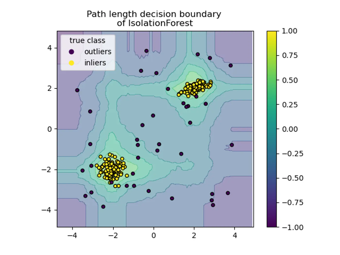
• Axis-Parallel Splits:
  • Standard iTrees 🌲 split only on one feature at a time, so:
    • We do not get a smooth decision boundary.
    • Anything off-axis has a higher probability of being marked as an outlier.
    • Note: Extended Isolation Forest fixes this by using random slopes.
• Score Sensitivity: The threshold for what constitutes an ‘anomaly’ often requires manual tuning or domain knowledge.

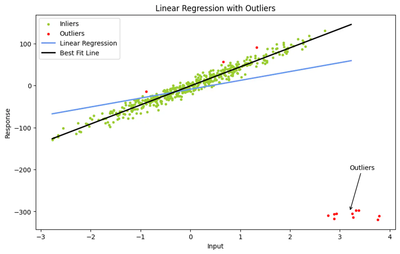
👉Ordinary Least Squares use all data points to find a fit.

• However, a single outlier can ‘pull’ the resulting line significantly, leading to a poor representative model.

💡If we pick a very small random subset of points, there is a higher probability that this small subset contains only good data (inliers) compared to a large set.

• Ordinary Least Squares (OLS) minimizes the Sum of Errors.

  • A huge outlier has an exponentially large impact on the final line.

  

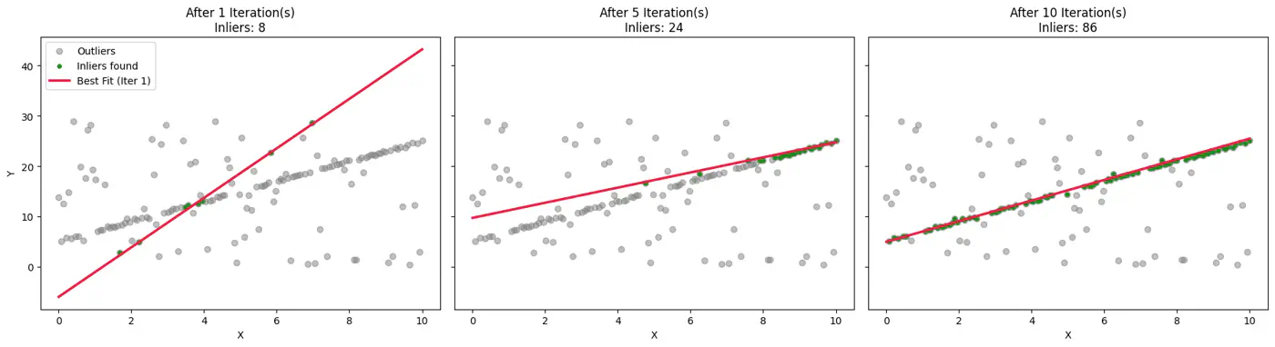
💡Instead of using all points, iteratively pick the smallest possible random subset to fit a model, then check (votes) how many other points in the dataset ‘agree’ with that model.

This gives the name to our algorithm:

• Random: Random subsets.
• Sampling: Small subsets.
• Consensus: Agreement with other points.

1. Random Sampling:
   • Randomly select a Minimal Sample Set (MSS) of ’n’ points from the input data ‘D’.
   • e.g. n=2 for a line, or n=3 for a plane in 3D.
2. Model Fitting:
   • Compute the model parameters using only these ’n’ points.
3. Test:
   • For all other points in ‘D’, calculate the error relative to the model.
   • 👉 Points with error < \(\tau\)(threshold) are added to the ‘Consensus Set’.
4. Evaluate:
   • If the consensus set is larger than the previous best, save this model and set.
5. Repeat 🔁:
   • Iterate ‘k’ times.
6. Refine (Optional):
   • Once the best model is found, re-estimate it using all points in the final consensus set (usually via Least Squares) for a more precise fit.

👉Example:

👉To ensure the algorithm finds a ‘clean’ sample set (no outliers) with a desired probability(often 99%), we use the following formula:

• k: Number of iterations required.
• P: Probability that at least one random sample contains only inliers.
• w: Ratio of inliers in the dataset (number of inliers / total points).
• n: Number of points in the Minimal Sample Set.