This is the multi-page printable view of this section. Click here to print.
Anomaly Detection
1 - Anomaly Detection
🦄 Anomaly is a rare item, event or observation which deviates significantly from the majority of the data and does not conform to a well-defined notion of normal behavior.
Note: Such examples may arouse suspicions of being generated by a different mechanism, or appear inconsistent with the remainder of that set of data.
Remove Outliers:
- Rejection or omission of outliers from the data to aid statistical analysis, for example to compute the mean or standard deviation of the dataset.
- Remove outliers for better predictions from models, such as linear regression.
Focus on Outliers:
- Fraud detection in banking and financial services.
- Cyber-security: intrusion detection, malware, or unusual user access patterns.
- Supervised
- Semi-Supervised
- ✅ Unsupervised (most common)
Note: Labeled anomaly data is often unavailable in real-world scenarios.
- Statistical Methods: Z-Score, large value means outlier, IQR, point beyond fences (Q1 - 1.5*IQR or Q3 + 1.5*IQR) is flagged as an outlier.
- Distance Based: KNN, points far from their neighbors as potential anomalies.
- Density Based: DBSCAN, points in low density regions are considered outliers.
- Clustering Based: K-Means, points far from cluster centroids that do not fit any cluster are anomalies.
- Elliptic Envelope (MCD - Minimum Covariance Determinant)
- One-Class SVM (OC-SVM)
- Local Outlier Factor (LOF)
- Isolation Forest (iForest)
- RANSAC (Random Sample Consensus)
2 - Elliptic Envelope
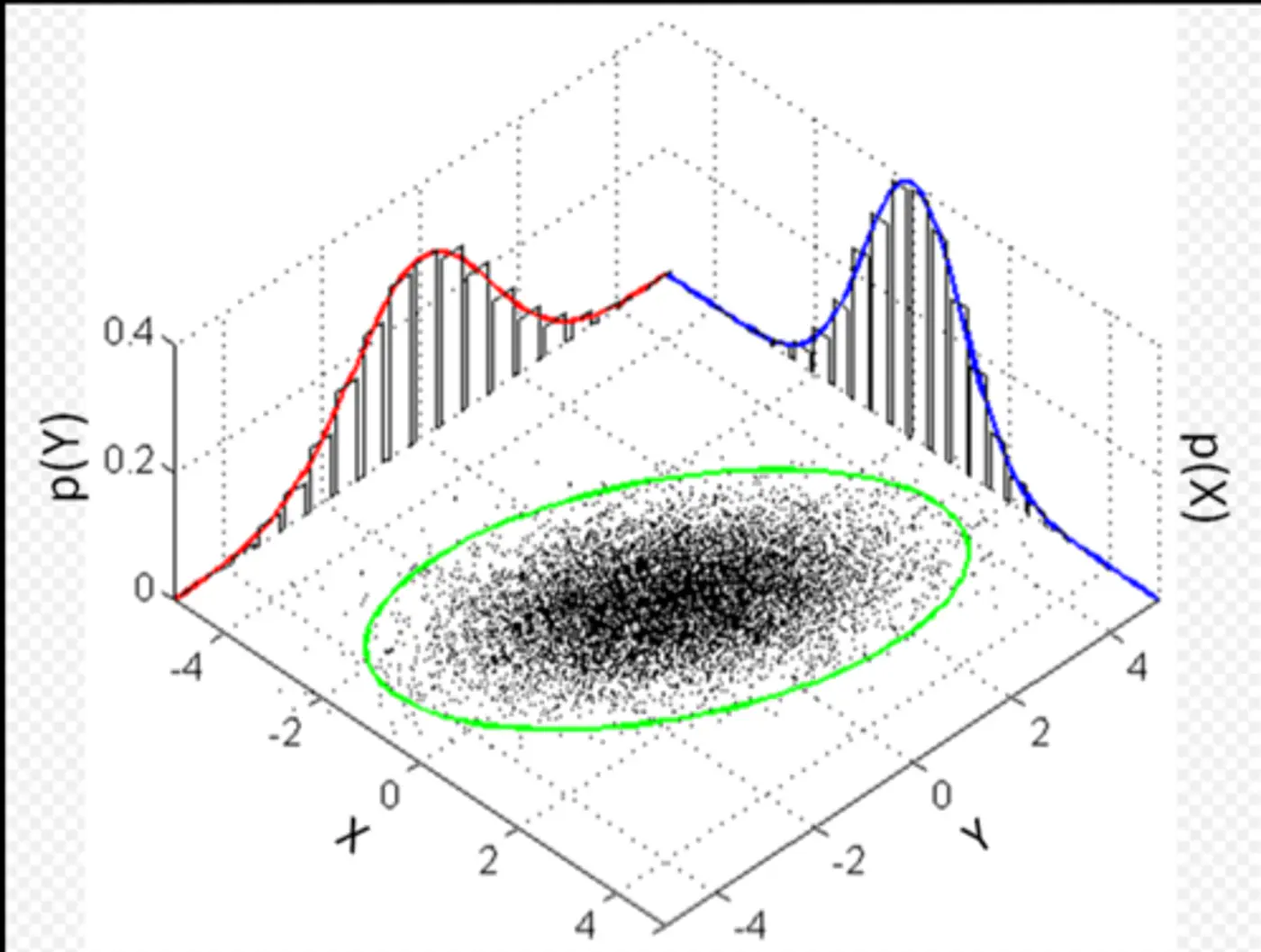
Detect anomalies in multivariate Gaussian data, such as, biometric data (height/weight) where features are normally distributed and correlated.
Assumption: The data can be modeled by a Gaussian distribution.
In a normal distribution, most data points cluster around the mean, and the probability density decreases as we move farther away from the center.
Euclidean distance measures the simple straight-line distance from the center of the cloud.
If the data is spherical, this works fine.
However, real-world data is often stretched or skewed (e.g., taller people are generally heavier), due to correlations between variables, forming an elliptical shape.
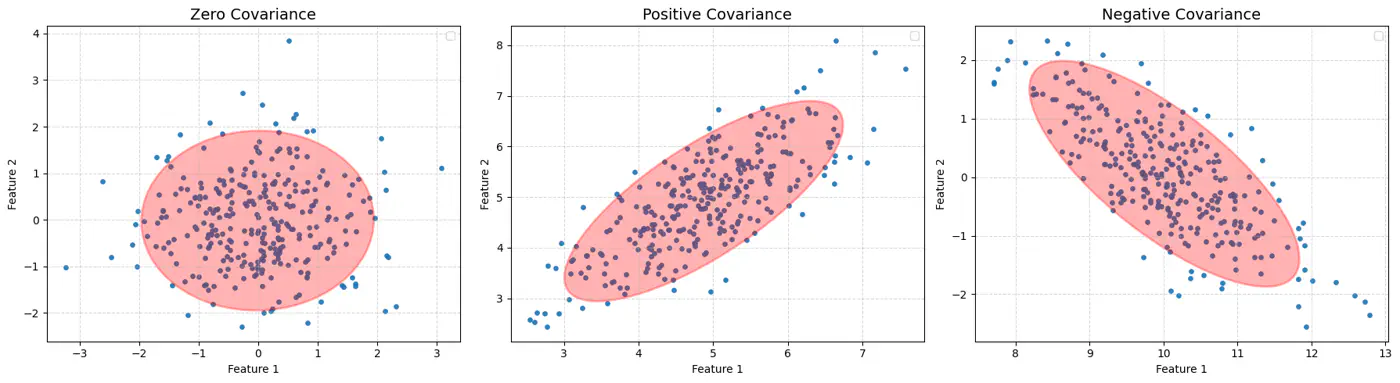
Mahalanobis distance essentially re-scales the data so that the elliptical distribution appears spherical, and then measures the Euclidean distance in that transformed space.
This way, it measures how many standard deviations(\(\sigma\)) away a point is from the mean, considering the data’s spread and correlation (covariance).
\[D_M(x) = \sqrt{(x - \mu)^T \Sigma^{-1} (x - \mu)}\]Find the most dense core of the data.
\[D_M(x) = \sqrt{(x - \mu)^T \Sigma^{-1} (x - \mu)}\]Determinant of covariance matrix \(\Sigma\) represents the volume of the ellipsoid.
Therefore, minimize \(|\Sigma|\) to find the tight core.
\(\text {Small} ~ \Sigma \rightarrow \text {Large} ~\Sigma ^{-1}\rightarrow \text {Large} ~ D_{M} ~\text {for outliers}\)
MCD algorithm is used to find the covariance matrix \(\Sigma\) with minimum determinant, so that the volume of the ellipsoid is minimized.
- Initialization: Select several random subsets of size h < n (default h = \(\frac{n+d+1}{2}\), d = # dimensions), representing ‘robust’ majority of the data.
- Calculate preliminary mean (\(\mu\)) and covariance (\(\Sigma\)) for each random subset.
- Concentration Step: Iterative core of the algorithm designed to ‘tighten’ the ellipsoid.
- Calculate Distances: Compute the Mahalanobis distance of all ’n’ points in the dataset from the current subset’s mean (\(\mu\)) and covariance (\(\Sigma\)).
- Select New Subset: Identify the ‘h’ points with the smallest Mahalanobis distances.
- These are the points most centrally located relative to the current ellipsoid.
- Update Estimates: Calculate a new and based only on these ‘h’ most central points.
- Repeat : The steps repeat until the determinant stops shrinking.
Note: Select the best subset that achieved the absolute minimum determinant.
- Assumptions
- Gaussian data.
- Unimodal data (single center).
- Cost of covariance matrix \(\Sigma^{-1}\) inversion is O(d^3).
3 - One Class SVM
Only one class of data (normal, non-outlier) is available for training, making standard supervised learning models impossible.
e.g. Only normal observations are available for fraud detection, cyber attack, fault detection etc.

The core problem is to build a model that can distinguish between ‘normal’ and ‘anomalous’ data when we only have examples of the ‘normal’ class during training.
We need to find a decision boundary that is as compact as possible while still encompassing the bulk of the training data.
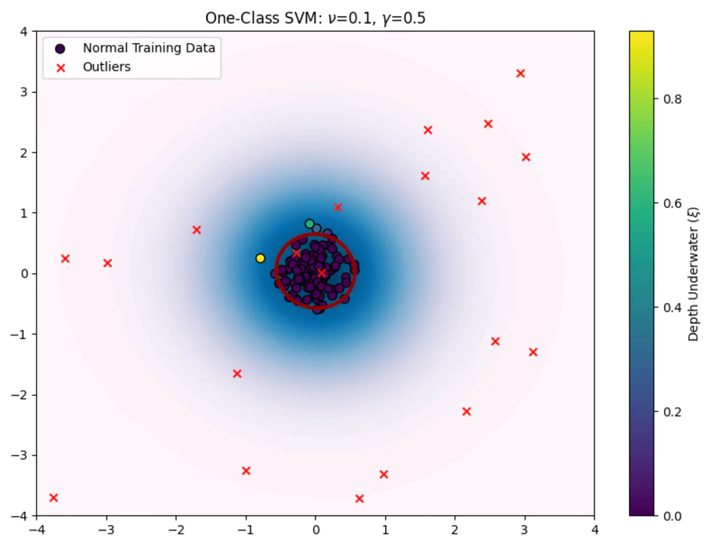
Define a boundary for a single class in high-dimensional space where data might be non-linearly distributed (e.g.‘U’ shape).
Use the Kernel Trick to project data into a higher-dimensional space and find a hyperplane that separates the data from the origin with the maximum margin.
OC-SVM, as introduced by Bernhard Schölkopf et al., uses a hyperplane ‘H’ defined by a weight vector \(\mathbf{w}\) and a bias term \(\rho\).
Solve the following optimization problem:
\[\min _{\mathbf{w},\xi _{i},\rho }\frac{1}{2}||\mathbf{w}||^{2}+\frac{1}{\nu N}\sum _{i=1}^{N}\xi _{i}-\rho \]Subject to constraints:
\[\mathbf{w}\cdot \phi (\mathbf{x}_{i})\ge \rho -\xi _{i}\quad \text{and}\quad \xi _{i}\ge 0,\quad \text{for\ }i=1,\dots ,N\]- \(\mathbf{x}_{i}\): i-th training data point.
- \(\phi (\mathbf{x}_{i})\): RBF kernel function \(K(x, y) = \exp(-\gamma \|x-y\|^2)\) that maps the data into a higher-dimensional feature space, making it easier to separate from the origin.
- \(\mathbf{w}\): normal vector to the separating hyperplane.
- \(\rho\): scalar bias term that determines the offset of the hyperplane from the origin.
- \(\xi_i\): Slack variables that allow some data points to fall on the ‘wrong’ side of the hyperplane (inside the anomalous region) to prevent overfitting.
- N: total number of training points.
- \(\nu\): hyper-parameter between 0 and 1. It acts as an upper bound on the fraction of outliers (training data points outside the boundary) and a lower bound on the fraction of support vectors.
- \(\frac{1}{2}\|\mathbf{w}\|^{2}\): aims to maximize the margin/compactness of the region.
- \(\frac{1}{\nu N}\sum _{i=1}^{N}\xi _{i}-\rho\): penalizes points (outliers) that violate the boundary constraints.
After solving the optimization problem using standard quadratic programming techniques, we obtain the optimal \(\mathbf{w}^{*}\) and \(\rho ^{*}\).
For a new data point \(x_{new}\), decision function is:
\[f(\mathbf{x}_{\text{new}})=\text{sign}(\mathbf{w}^{*}\cdot \phi (\mathbf{x}_{\text{new}})-\rho ^{*})\]\(f(\mathbf{x}_{\text{new}})\ge 0\): normal point.
\(f(\mathbf{x}_{\text{new}})< 0\): anomalous point (outlier).
4 - Local Outlier Factor
A $100 transaction might be ‘normal’ in New York but an ‘outlier’ in a small rural village.
‘Local context matters.’
Global distance metrics fail when density is non-uniform.
An outlier is a point that is ‘unusual’ relative to its immediate neighbors, regardless of how far it is from the center of the entire dataset.
Traditional distance-based outlier detection methods, such as, KNN, often struggle with datasets where data is clustered at varying densities.
- A point in a sparse region might be considered an outlier by a global method, even if it is a normal part of that sparse cluster.
- Conversely, a point very close to a dense cluster might be an outlier relative to that specific neighborhood.
Calculate the relative density of a point compared to its immediate neighborhood.
e.g. If the neighbors are in a dense crowd and the point is not, it is an outlier.
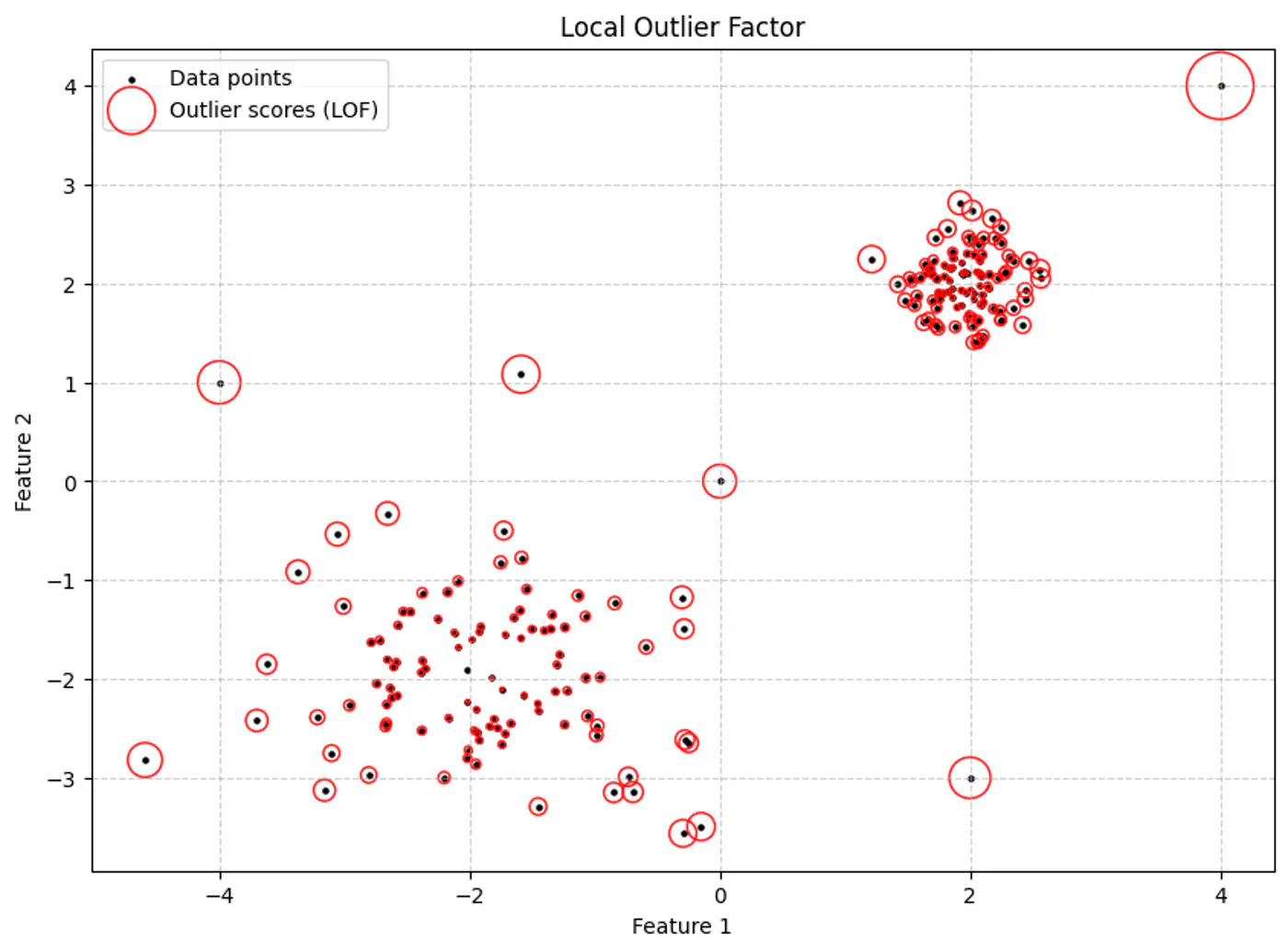
Local Outlier Factor (LOF) is a density-based algorithm designed to detect anomalies by measuring the local deviation of a data point relative to its neighbors.
Size of the red circle represents the LOF score.
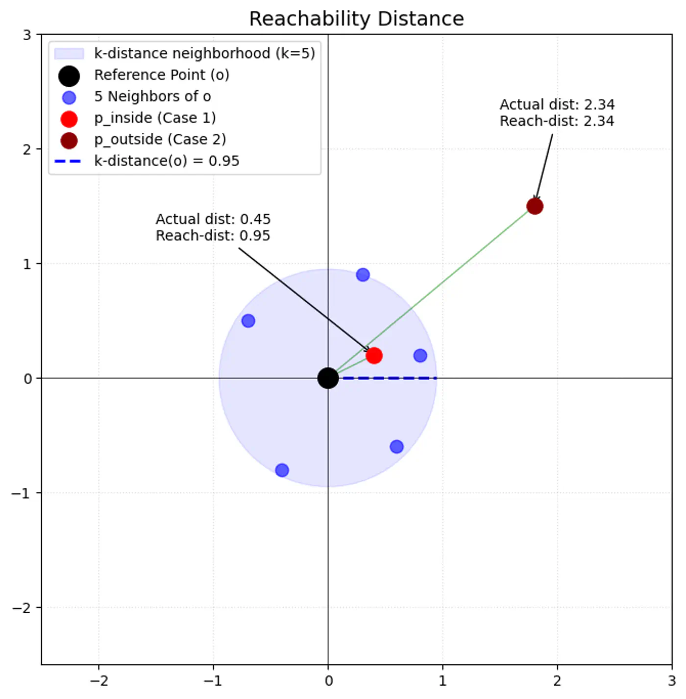
- K-Distance (\(k\text{-dist}(p)\)):
- The distance from point ‘p’ to its k-th nearest neighbor.
- Reachability Distance (\(\text{reach-dist}_{k}(p,o)\)):
\[\text{reach-dist}_{k}(p,o)=\max \{k\text{-dist}(o),\text{dist}(p,o)\}\]
- \(\text{dist}(p,o)\): actual Euclidean distance between ‘p’ and ‘o’.
- This acts as ‘smoothing’ factor.
- If point ‘p’ is very close to ‘o’ (inside o’s k-neighborhood), round up distance to \(k\text{-dist}(o)\).
- \(\text{dist}(p,o)\): actual Euclidean distance between ‘p’ and ‘o’.
- Local Reachability Density (\(\text{lrd}_{k}(p)\)):
- The inverse of the average reachability distance from ‘p’ to its k-neighbors (\(N_{k}(p)\)).
\[\text{lrd}_{k}(p)=\left[\frac{1}{|N_{k}(p)|}\sum _{o\in N_{k}(p)}\text{reach-dist}_{k}(p,o)\right]^{-1}\]
- High LRD: Neighbors are very close; the point is in a dense region.
- Low LRD: Neighbors are far away; the point is in a sparse region.
- The inverse of the average reachability distance from ‘p’ to its k-neighbors (\(N_{k}(p)\)).
\[\text{lrd}_{k}(p)=\left[\frac{1}{|N_{k}(p)|}\sum _{o\in N_{k}(p)}\text{reach-dist}_{k}(p,o)\right]^{-1}\]
- Local Outlier Factor (\(\text{LOF}_{k}(p)\)):
- The ratio of the average ‘lrd’ of p’s neighbors to p’s own ‘lrd’. \[\text{LOF}_{k}(p)=\frac{1}{|N_{k}(p)|}\sum _{o\in N_{k}(p)}\frac{\text{lrd}_{k}(o)}{\text{lrd}_{k}(p)}\]
- LOF ≈ 1: Point ‘p’ has similar density to its neighbors (inlier).
- LOF > 1: Point p’s density is much lower than its neighbors’ density (outlier).
5 - Isolation Forest
‘Large scale tabular data.’
Credit card fraud detection in datasets with millions of rows and hundreds of features.
Note: Supervised learning requires balanced, labeled datasets (normal vs. anomaly), which are rarely available in real-world scenarios like fraud or cyber-attacks.
‘Flip the logic.’
‘Anomalies’ are few and different, so they are much easier to isolate from the rest of the data than normal points.
‘Curse of dimensionality.’
Distance based (K-NN), and density based (LOF) algorithms require calculation of distance between all pair of points.
As the number of dimensions and data points grows, these calculations become exponentially more expensive and less effective.
‘Randomly partition the data.’
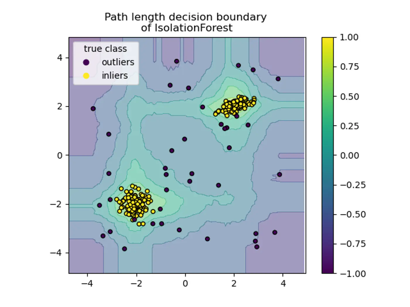
If a point is an outlier, it will take fewer partitions (splits) to isolate it into a leaf node compared to a point that is buried deep within a dense cluster of normal data.
Isolation Forest uses an ensemble of ‘Isolation Trees’ (iTrees) .
iTree (Isolation Tree) is a proper binary tree structure specifically designed to separate individual data points through random recursive partitioning.
- Sub-sampling:
- Select a random subset of data (typically 256 instances) to build an iTree.
- Tree Construction: Randomly select a feature.
- Randomly select a split value between the minimum and maximum values of that feature.
- Divide the data into two branches based on this split.
- Repeat recursively until the point is isolated or a height limit is reached.
- Forest Creation:
- Repeat the process to create ‘N’ trees (typically 100).
- Inference:
- Pass a new data point through all trees, calculate the average path length, and compute the anomaly score.
Assign an anomaly score based on the path length h(x) required to isolate a point ‘x’.
- Path Length (h(x)): The number of edges ‘x’ traverses from the root node to a leaf node.
- Average Path Length (c(n)): Since iTrees are structurally similar to Binary Search Trees (BST), the average path length for a dataset of size ’n’ is given by: \[c(n)=2H(n-1)-\frac{2(n-1)}{n}\]
where, H(i) is the harmonic number, estimated as \(\ln (i)+0.5772156649\) (Euler’s constant).
To normalize the score between 0 and 1, we define it as:
\[s(x,n)=2^{-\frac{E(h(x))}{c(n)}}\]E(H(x)): is the average path length of across a forest of trees .
- \(s\rightarrow 1\): Point is an anomaly; Path length is very short.
- \(s\approx 0.5\): Point is normal, path length approximately equal to c(n).
- \(s\rightarrow 0\): Point is normal; deeply buried point, path length is much larger than c(n).
- Axis-Parallel Splits:
- Standard iTrees split only on one feature at a time, so:
- We do not get a smooth decision boundary.
- Anything off-axis has a higher probability of being marked as an outlier.
- Note: Extended Isolation Forest fixes this by using random slopes.
- Standard iTrees split only on one feature at a time, so:
- Score Sensitivity: The threshold for what constitutes an ‘anomaly’ often requires manual tuning or domain knowledge.
6 - RANSAC
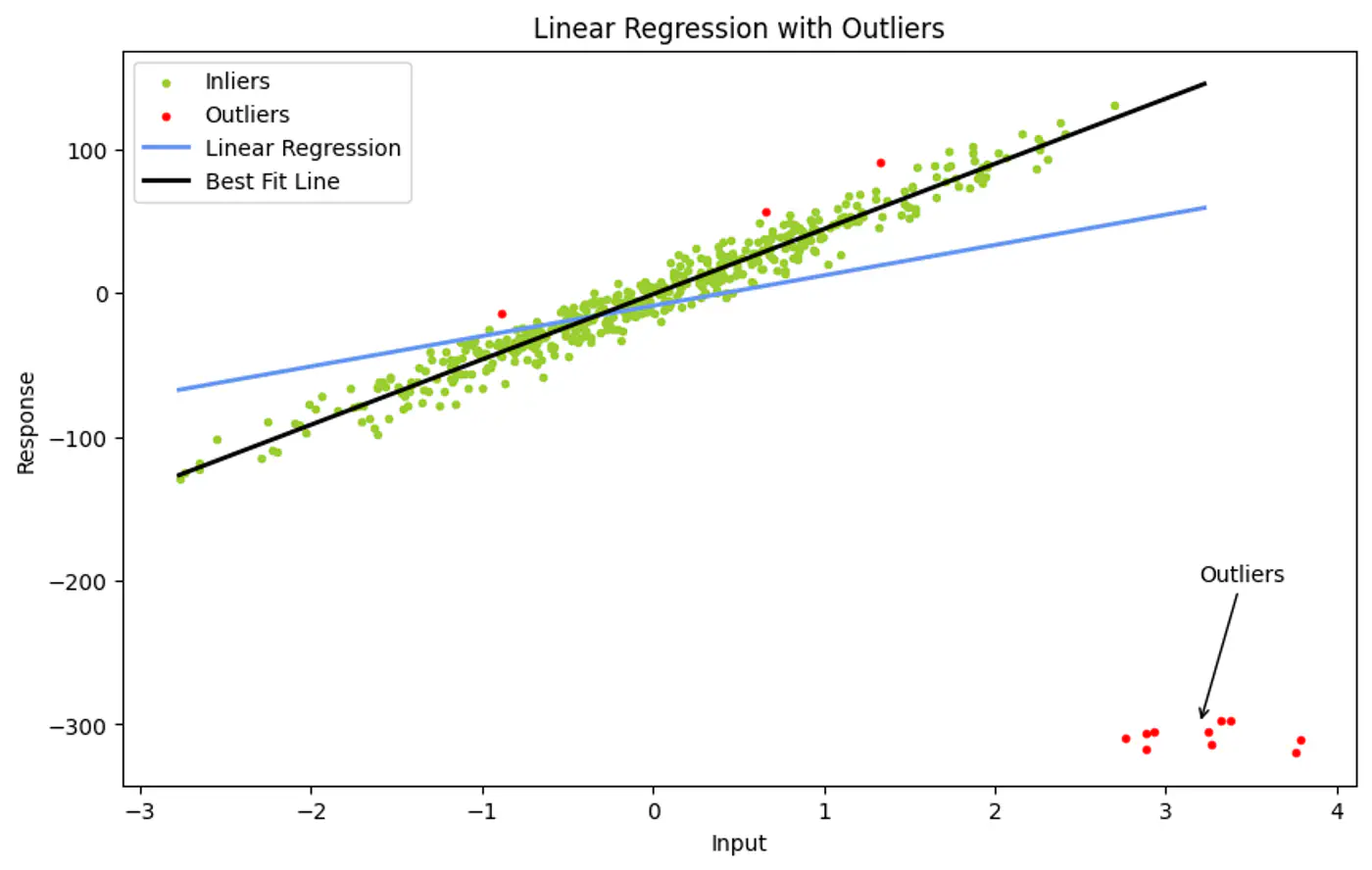
Ordinary Least Squares use all data points to find a fit.
- However, a single outlier can ‘pull’ the resulting line significantly, leading to a poor representative model.
If we pick a very small random subset of points, there is a higher probability that this small subset contains only good data (inliers) compared to a large set.
Ordinary Least Squares (OLS) minimizes the Sum of Errors.
- A huge outlier has an exponentially large impact on the final line.
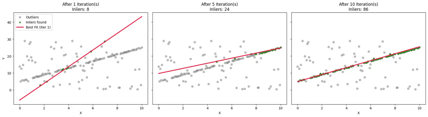
Instead of using all points, iteratively pick the smallest possible random subset to fit a model, then check (votes) how many other points in the dataset ‘agree’ with that model.
This gives the name to our algorithm:
- Random: Random subsets.
- Sampling: Small subsets.
- Consensus: Agreement with other points.
- Random Sampling:
- Randomly select a Minimal Sample Set (MSS) of ’n’ points from the input data ‘D’.
- e.g. n=2 for a line, or n=3 for a plane in 3D.
- Model Fitting:
- Compute the model parameters using only these ’n’ points.
- Test:
- For all other points in ‘D’, calculate the error relative to the model.
- Points with error < \(\tau\)(threshold) are added to the ‘Consensus Set’.
- Evaluate:
- If the consensus set is larger than the previous best, save this model and set.
- Repeat :
- Iterate ‘k’ times.
- Refine (Optional):
- Once the best model is found, re-estimate it using all points in the final consensus set (usually via Least Squares) for a more precise fit.
Example:
To ensure the algorithm finds a ‘clean’ sample set (no outliers) with a desired probability(often 99%), we use the following formula:
\[k=\frac{\log (1-P)}{\log (1-w^{n})}\]- k: Number of iterations required.
- P: Probability that at least one random sample contains only inliers.
- w: Ratio of inliers in the dataset (number of inliers / total points).
- n: Number of points in the Minimal Sample Set.