This is the multi-page printable view of this section. Click here to print.
Dimensionality Reduction
1 - PCA
- Data Compression
- Noise Reduction
- Feature Extraction: Create a smaller set of meaningful features from a larger one.
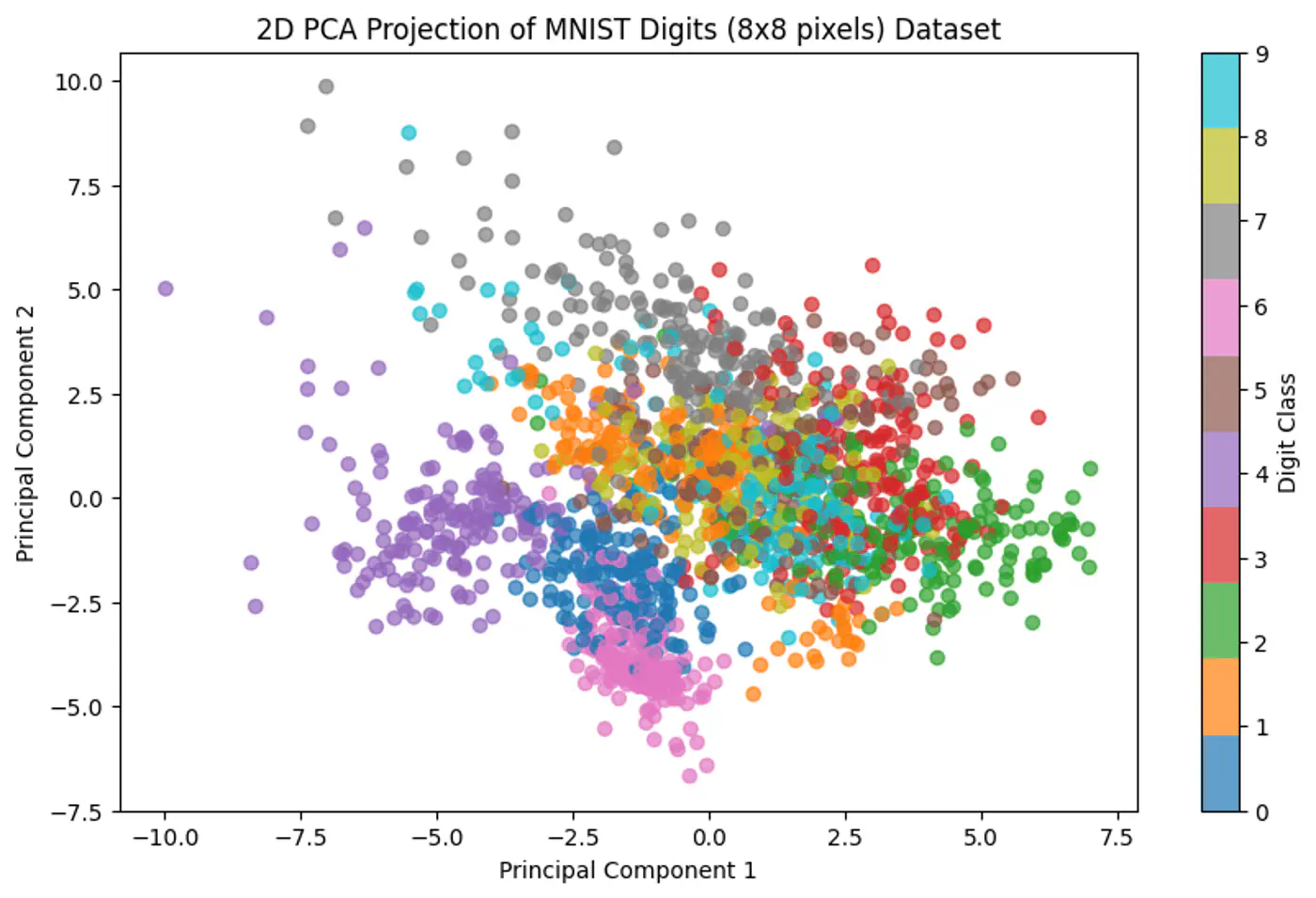
- Data Visualization: Project high-dimensional data down to 2 or 3 dimensions.
Assumption: Linear relationship between features.
‘Information = Variance’
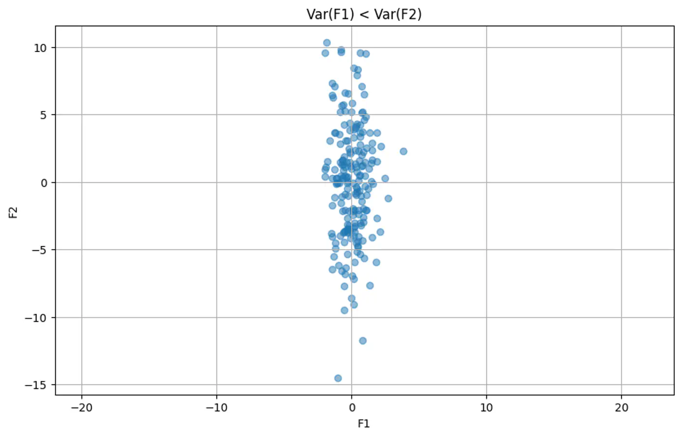
Imagine a cloud of points in 2D space.
Look for the direction (axis) along which the data is most ‘spread out’.
By projecting data onto this axis, we retain the maximum amount of information (variance).
Example 1: Var(Feature 1) < Var(Feature 1)
Example 2: Red line shows the direction of maximum variance
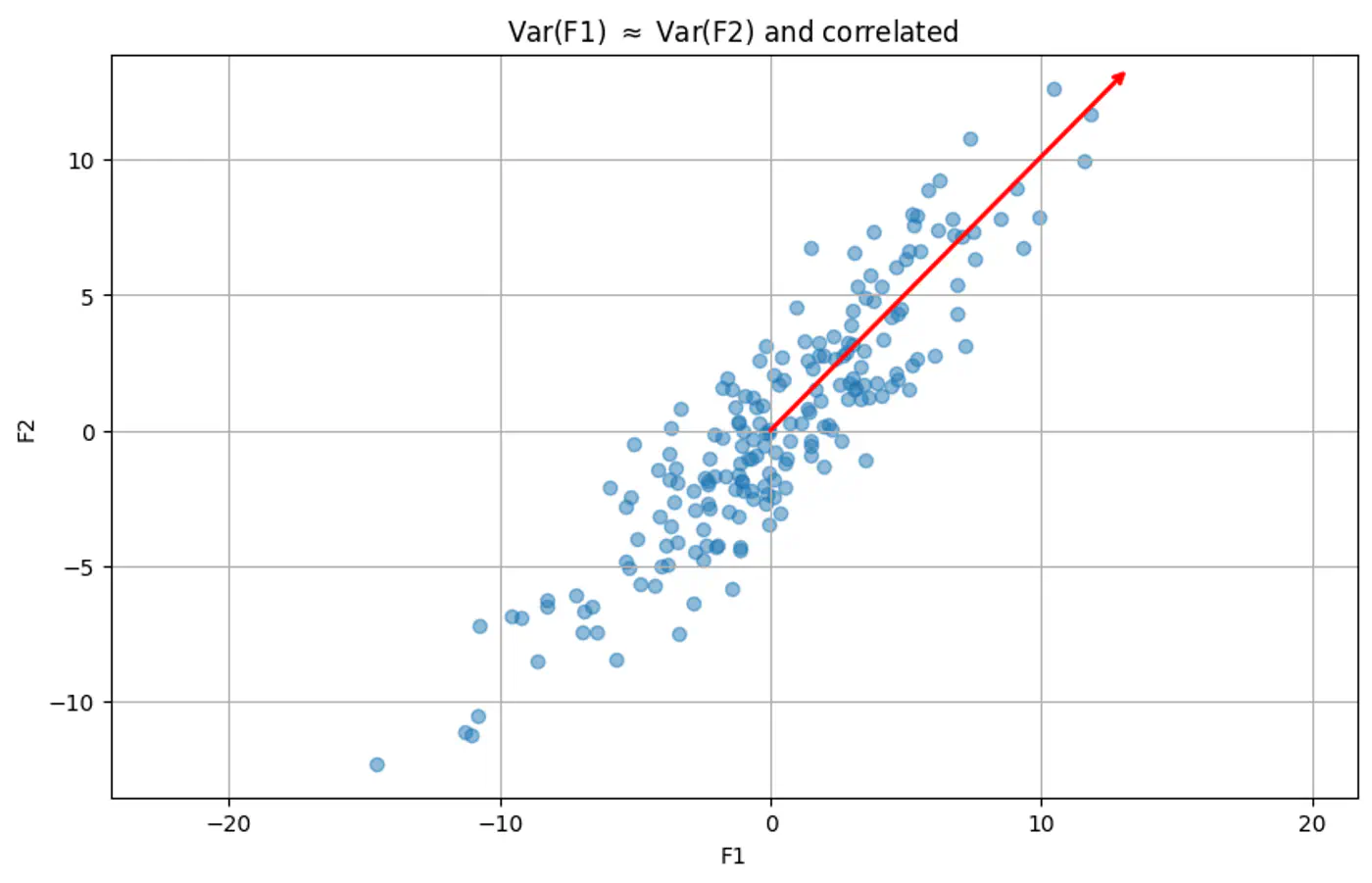
Finds the direction of maximum variance in the data.
Note: Some loss of information will always be there in dimensionality reduction, because there will be some variability in data along the direction that is dropped, and that will be lost.
- PCA seeks a direction , represented by a unit vector \(\hat{u}\) onto which data can be projected to maximize variance.
- The projection of a mean centered data point \(x_i\) onto \(u\) is \(u^Tx_i\).
- The variance of these projections can be expressed as \(u^{T}\Sigma u\), where \(\Sigma\) is the data’s covariance matrix.
- Data: Let \(X = \{x_{1},x_{2},\dots ,x_{n}\}\) is the mean centered (\(\bar{x} = 0\)) dataset.
- Projection of point \(x_i\) on \(u\) is \(z_i = u^Tx_i\)
- Variance of projected points (since \(\bar{x} = 0\)): \[\text{Var}(z)=\frac{1}{n}\sum _{i=1}^{n}z_{i}^{2}=\frac{1}{n}\sum _{i=1}^{n}(x_{i}^{T}u)^{2}\]
- Since, \((x_{i}^{T}u)^{2} = (u^{T}x_{i})(x_{i}^{T}u)\) \( \implies\text{Var}(z)=u^{T}\left(\frac{1}{n}\sum _{i=1}^{n}x_{i}x_{i}^{T}\right)u\)
- Since, Covariance Matrix, \(\Sigma = \left(\frac{1}{n}\sum _{i=1}^{n}x_{i}x_{i}^{T}\right)\)
- Therefore, \(\text{Var}(z)=u^{T}\Sigma u\)
To prevent infinite variance, PCA constrains \(u\) to be a unit vector (\(\|u\|=1\)).
\[\text{maximize\ }u^{T}\Sigma u, \quad \text{subject\ to\ }u^{T}u=1\]Note: This constraint forces the optimization algorithm to focus purely on the direction that maximizes variance, rather than allowing it to artificially inflate the variance by increasing the length of the vector.
Lagrangian function: \(L(u,\lambda )=u^{T}\Sigma u-\lambda (u^{T}u-1)\)
To find \(u\) that maximizes above constrained optimization:
This is the standard Eigenvalue Equation.
So, the optimal directions \(u\) are the eigenvectors of the covariance matrix \(\Sigma\).
To see which eigenvector maximizes variance, substitute the result back into the variance equation:
\[\text{Variance}=u^{T}\Sigma u=u^{T}(\lambda u)=\lambda (u^{T}u)=\lambda \]Since the variance equals the eigenvalue \(\lambda\), the direction \(u\) that maximizes variance is the eigenvector associated with the largest eigenvalue.
- Center the data: \(X = X - \mu\)
- Compute the Covariance Matrix: \(\Sigma = \frac{1}{n-1} X^T X\)
- Compute Eigenvectors and Eigenvalues of \(\Sigma\) .
- Sort eigenvalues in descending order and select the top ‘k’ eigenvectors.
- Project the original data onto the subspace: \(Z = X W_k\) where, \(W_{k}=[u_{1},u_{2},\dots ,u_{k}]\) , matrix formed by ‘k’ eigenvectors corresponding to ‘k’ largest eigenvalues.
- Cannot model non-linear relationships.
- Sensitive to outliers.
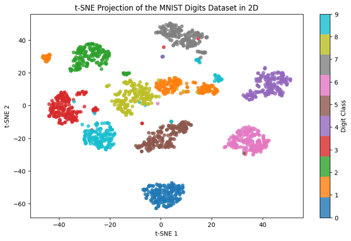
2 - t-SNE
PCA preserves variance, not neighborhoods.
t-SNE focuses on the ‘neighborhood’ (local structure).
Tries to keep points that are close together in high-dimensional space close together in low-dimensional space.
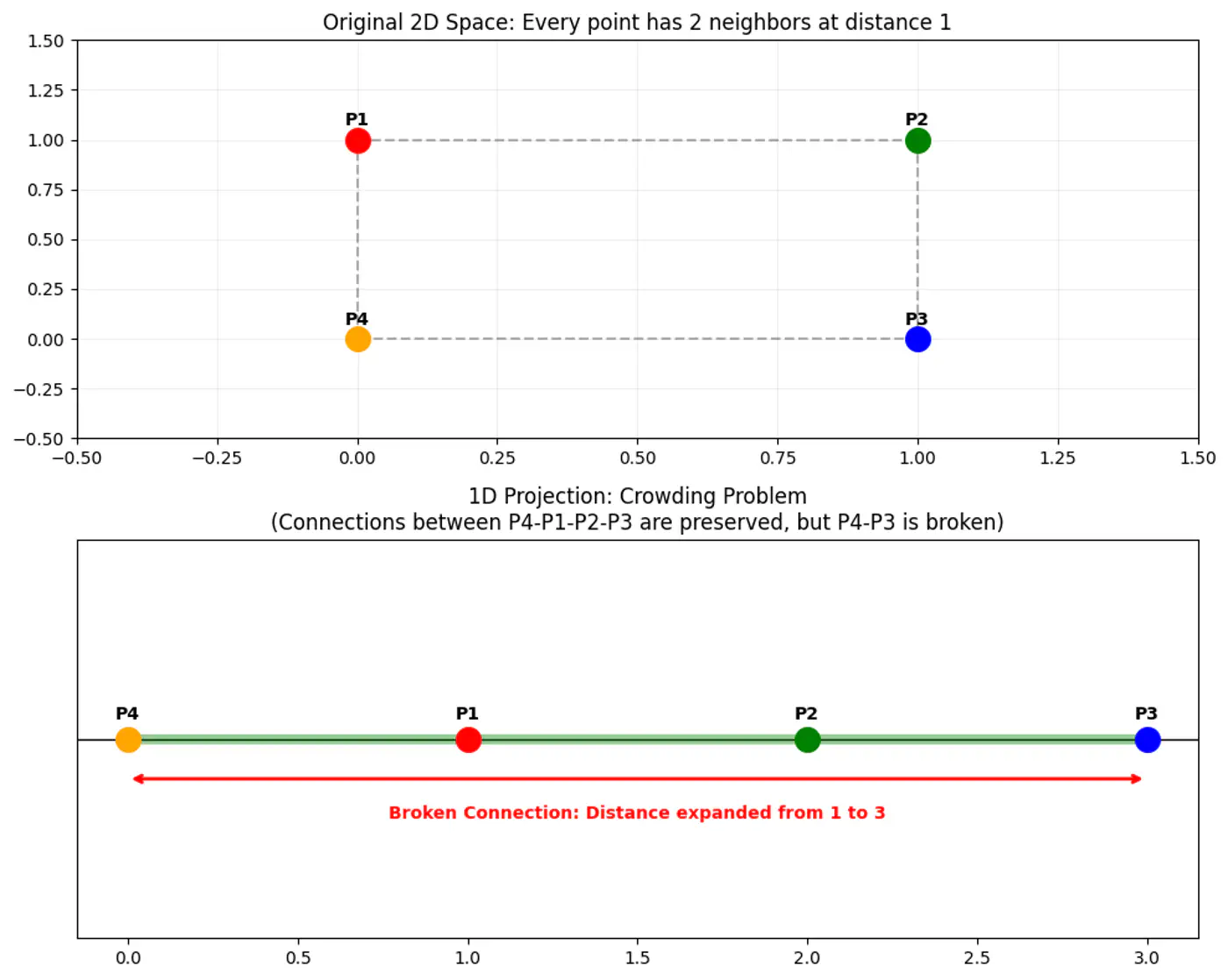
Map high-dimensional points to low-dimensional points , such that the pairwise similarities are preserved, while solving the ‘crowding problem’ (where points collapse into a single cluster).
Crowding Problem
Convert Euclidean distances into conditional probabilities representing similarities.
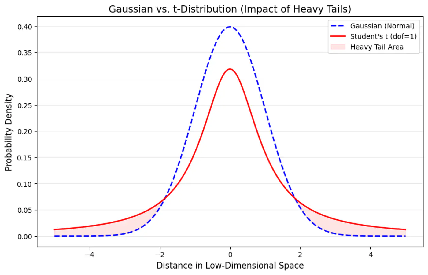
Minimize the divergence between the probability distributions of the high-dimensional (Gaussian) and low-dimensional (t-distribution) spaces.
Note: Probabilistic approach to defining neighbors is the core ‘stochastic’ element of the algorithm’s name.
The similarity of datapoint \(x_j\) to datapoint \(x_i\) is the conditional probability \(p_{j|i}\), that \(x_i\) would pick \(x_j\) as its neighbor.
Note: If neighbors are picked in proportion to their probability density under a Gaussian centered at \(x_i\).
\[p_{j|i} = \frac{\exp(-||x_i - x_j||^2 / 2\sigma_i^2)}{\sum_{k \neq i} \exp(-||x_i - x_k||^2 / 2\sigma_i^2)}\]- \(p_{j|i}\) high: nearby points.
- \(p_{j|i}\) low: widely separated points.
Note: Make probabilities symmetric: \(p_{ij} = \frac{p_{j|i} + p_{i|j}}{2n}\)
To solve the crowding problem, we use a heavy-tailed distribution (Student’s-t distribution with degree of freedom \(\nu=1\)).
\[q_{ij} = \frac{(1 + ||y_i - y_j||^2)^{-1}}{\sum_{k \neq l} (1 + ||y_k - y_l||^2)^{-1}}\]Note: Heavier tail spreads out dissimilar points more effectively, allowing moderately distant points to be mapped further apart, preventing clusters from collapsing and ensuring visual separation and cluster distinctness.
Measure the difference between the distributions ‘p’ and ‘q’ using the Kullback-Leibler (KL) divergence, which we aim to minimize:
\[C = KL(P||Q) = \sum_i \sum_j p_{ij} \log \frac{p_{ij}}{q_{ij}}\]Use gradient descent to iteratively adjust the positions of the low-dimensional points \(y_i\).
The gradient of the KL divergence is:
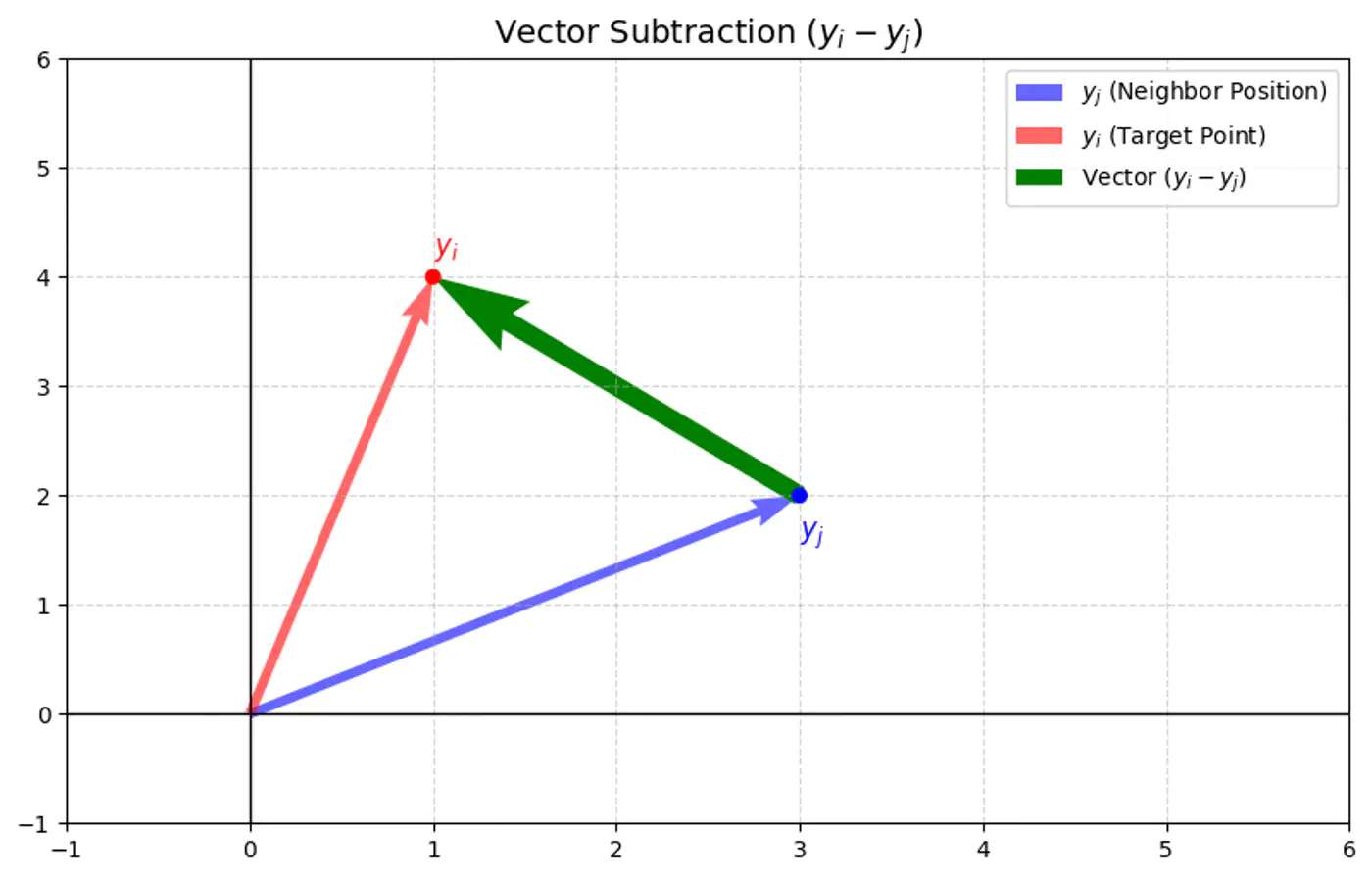
\[\frac{\partial C}{\partial y_{i}}=4\sum _{j\ne i}(p_{ij}-q_{ij})(y_{i}-y_{j})(1+||y_{i}-y_{j}||^{2})^{-1}\]- C : t-SNE cost function (sum of all KL divergences).
- \(y_i, y_j\): coordinates of data points and in the low-dimensional space (typically 2D or 3D).
- \(p_{ij}\): high-dimensional similarity (joint probability) between points \(x_i\) and \(x_j\), calculated using a Gaussian distribution.
- \(q_{ij}\): low-dimensional similarity (joint probability) between points \(y_i\) and \(y_j\), calculated using a Student’s t-distribution with one degree of freedom.
- \((1+||y_{i}-y_{j}||^{2})^{-1}\): term comes from the heavy-tailed Student’s t-distribution, which helps mitigate the ‘crowding problem’ by allowing points that are moderately far apart to have a small attractive force.
The gradient can be understood as a force acting on each point \(y_i\) in the low-dimensional map:
\[\frac{\partial C}{\partial y_{i}}=4\sum _{j\ne i}(p_{ij}-q_{ij})(y_{i}-y_{j})(1+||y_{i}-y_{j}||^{2})^{-1}\]- Attractive forces: If \(p_{ij}\) is large ⬆️ and \(q_{ij}\) is small ⬇️ (meaning two points were close in the high-dimensional space but are far in the low-dimensional space), the term \((p_{ij}-q_{ij})\) is positive, resulting in a strong attractive force pulling \(y_i\) and \(y_j\) closer.
- Repulsive forces: If \(p_{ij}\) is small ⬇️ and \(q_{ij}\) is large ⬆️ (meaning two points were far in the high-dimensional space but are close in the low-dimensional space), the term \((p_{ij}-q_{ij})\) is negative, resulting in a repulsive force pushing \(y_i\) and \(y_j\) apart.
Update step of in low dimensions:
\[y_{i}^{(t+1)}=y_{i}^{(t)}-\eta \frac{\partial C}{\partial y_{i}}\]Attractive forces (\(p_{ij}>q_{ij}\)):
- The negative gradient moves \(y_i\) opposite to the (\(y_i - y_j\)) vector, pulling it toward \(y_j\).
Repulsive forces (\(p_{ij} < q_{ij}\)):
- The negative gradient moves \(y_i\) in the same direction as the (\(y_i - y_j\)) vector, pushing it away from \(y_j\).
User-defined parameter that loosely relates to the effective number of neighbors.
Note: Variance \(\sigma_i^2\) (Gaussian) is adjusted for each point to maintain a consistent perplexity.
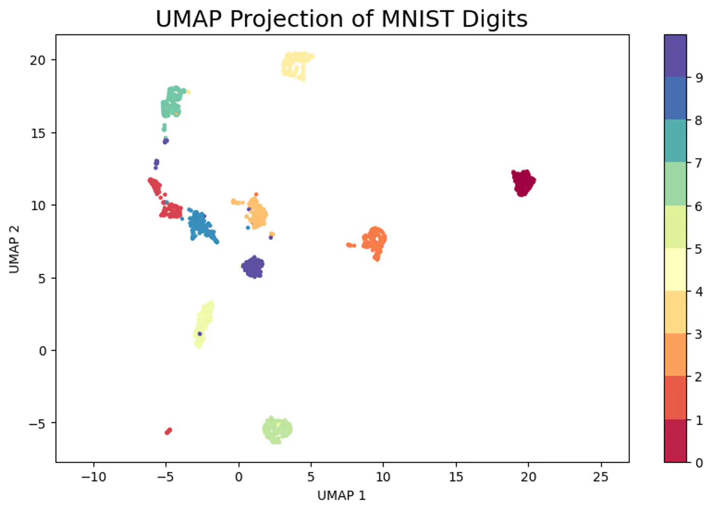
3 - UMAP
Visualizing massive datasets where t-SNE is too slow.
Creating robust low-dimensional inputs for subsequent machine learning models.
Using a world map ️ (2D)instead of globe for spherical(3D) earth .
It preserves the neighborhood relationships of countries (e.g., India is next to China), and to a good degree, the global structure.
Non-linear dimensionality reduction technique to visualize high-dimensional data (like images, gene expressions) in a lower-dimensional space (typically 2D or 3D), preserving its underlying structure and relationships.
Constructs a high-dimensional graph of data points and then optimizes a lower-dimensional layout to closely match this graph, making complex datasets understandable by revealing patterns, clusters, and anomalies.
Note: Similar to t-SNE but often faster and better at maintaining global structure.
Create a weighted graph (fuzzy simplicial set) representing the data’s topology and then find a low-dimensional graph that is as structurally similar as possible.
Note: Fuzzy means instead of using binary 0/1, we use weights in the range [0,1] for each edge.
- UMAP determines local connectivity based on a user-defined number of neighbors (n_neighbors).
- Normalizes distances locally using the distance to the nearest neighbor (\(\rho_i\)) and a scaling factor (\(\sigma_i\)) adjusted to enforce local connectivity constraints.
- The weight \(W_{ij}\) (fuzzy similarity) in high-dimensional space is: \[W_{ij}=\exp \left(-\frac{\max (0,\|x_{i}-x_{j}\|-\rho _{i})}{\sigma _{i}}\right)\]
Note: This ensures that the closest point always gets a weight of 1, preserving local structure.
In the low-dimensional space (e.g., 2D), UMAP uses a simple curve (similar to the t-distribution used in t-SNE) for edge weights:
\[Z_{ij}=(1+a\|y_{i}-y_{j}\|^{2b})^{-1}\]Note: The parameters ‘a’ and ‘b’ are typically fixed based on the ‘min_dist’ user parameter (e.g. min_dist = 0.1, then a≈1,577, b≈0.895).
Unlike t-SNE’s KL divergence, UMAP minimizes the cross-entropy between the high-dimensional weights \(W_{ij}\) and the low-dimensional weights \(Z_{ij}\).
Cost Function (C):
\[C=\sum _{i,j}\left(W_{ij}\log \frac{W_{ij}}{Z_{ij}}+(1-W_{ij})\log \frac{1-W_{ij}}{1-Z_{ij}}\right)\]Cost Function (C):
\[C=\sum _{i,j}\left(W_{ij}\log \frac{W_{ij}}{Z_{ij}}+(1-W_{ij})\log \frac{1-W_{ij}}{1-Z_{ij}}\right)\]Goal : Reduce overall Cross Entropy Loss.
- Attractive Force: \(W_{ij}\) high; make \(Z_{ij}\) high to make the log \(\frac{W_{ij}}{Z_{ij}} \)term small.
- Repulsive Force: \(W_{ij}\) low; make \(Z_{ij}\) low to make the \(log\frac{1-W_{ij}}{1-Z_{ij}}\) term small.
Note: This push and pull of 2 ‘forces’ will make the data in low dimensions settle into a position that is overall a good representation of the original data in higher dimensions.
- Mathematically complex.
- Requires tuning (n_neighbors, min_dist).