This is the multi-page printable view of this section. Click here to print.
Gaussian Mixture Model
1 - Gaussian Mixture Models
K-means uses Euclidean distance and assumes that clusters are spherical (isotropic) and have the same variance across all dimensions.
Places a circle or sphere around each centroid.
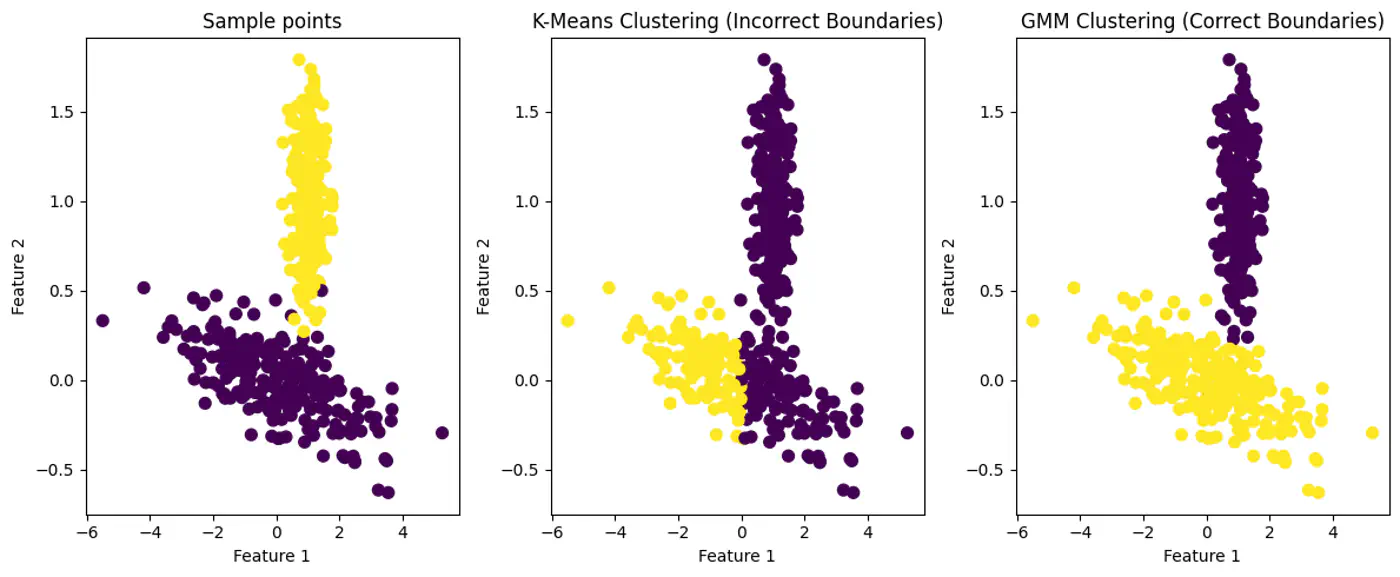
- What if the clusters are elliptical ? K-Means Fails with Elliptical Clusters.
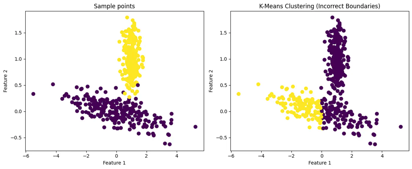
GMM: ‘Probabilistic evolution’ of K-Means
GMM provides soft assignments and can model elliptical clusters by accounting for variance and correlation between features.
Note: GMM assumes that all data points are generated from a mixture of a finite number of Gaussian Distributions with unknown parameters.
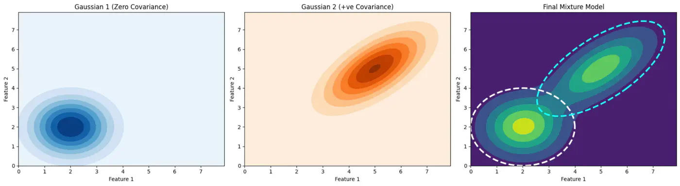
GMM can Model Elliptical Clusters.
‘Combination of probability distributions’.
Soft Assignment: Instead of a simple ‘yes’ or ’no’ for cluster membership, a data point is assigned a set of probabilities, one for each cluster.
e.g: A data point might have a 60% probability of belonging to cluster ‘A’, 30% probability for cluster ‘B’, and 10% probability for cluster ‘C’.
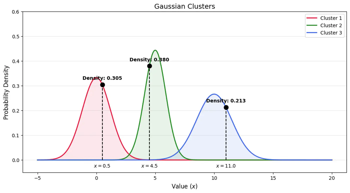
Gaussian Mixture Model Example:
Note: The term \(1/(\sqrt{2\pi \sigma ^{2}})\) is a normalization constant to ensure the total area under the curve = 1.
Multivariate Gaussian Example:
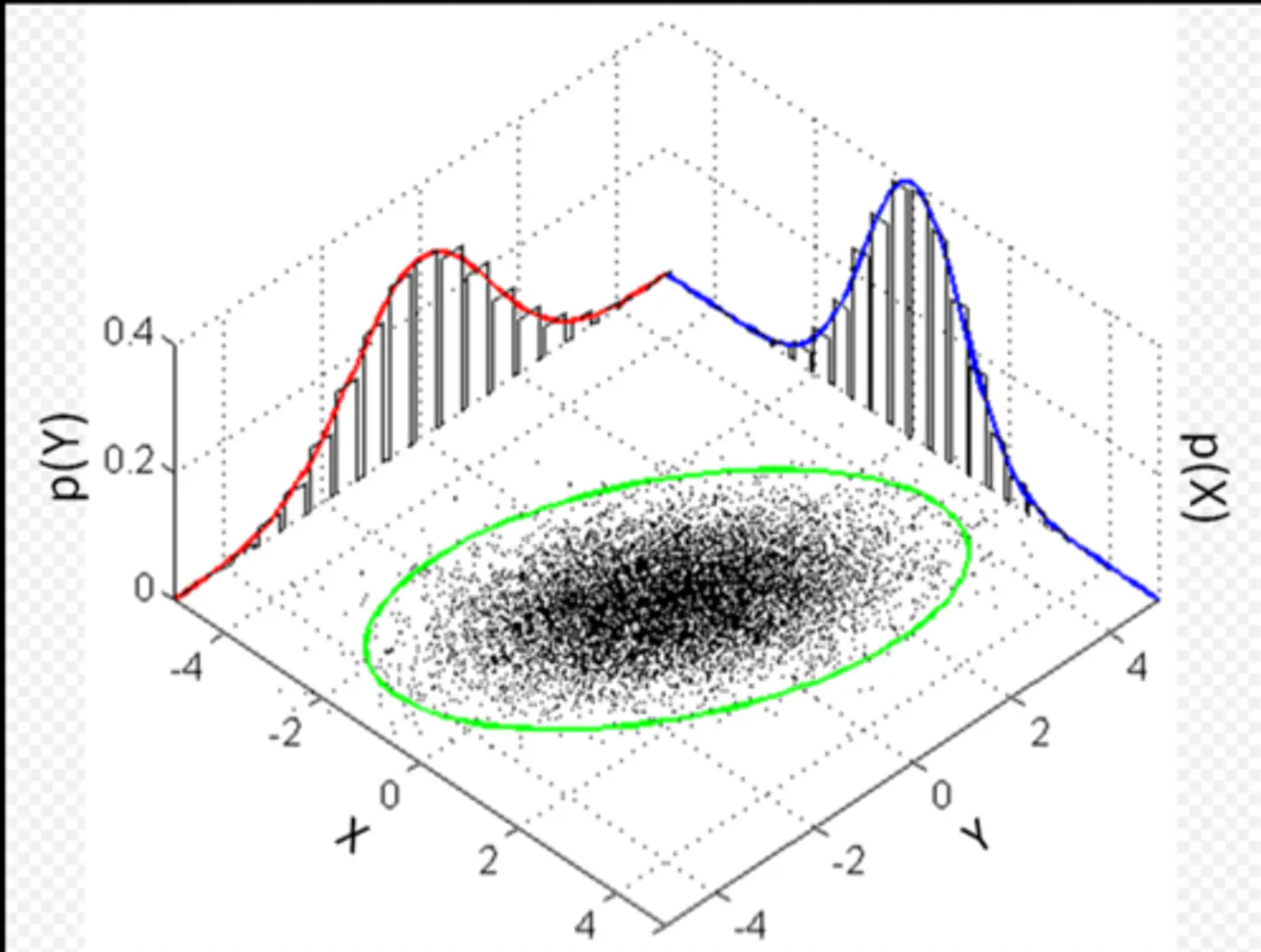
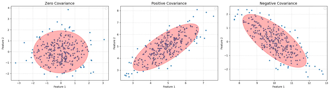
Whenever we have multivariate Gaussian, then the variables may be independent or correlated.
Feature Covariance:
Gaussian Mixture with PDF
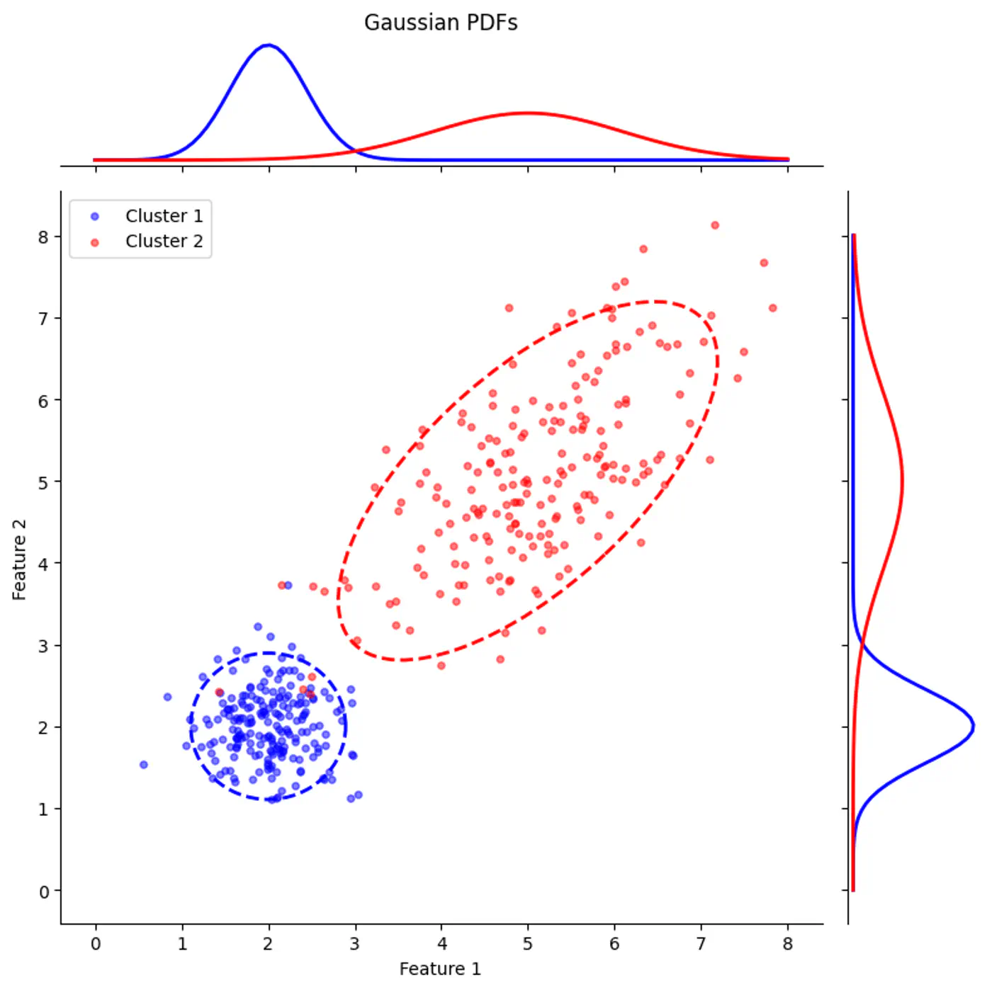
Gaussian Mixture (2D)
2 - Latent Variable Model
Probabilistic model that assumes data is generated from a mixture of several Gaussian (normal) distributions with unknown parameters.
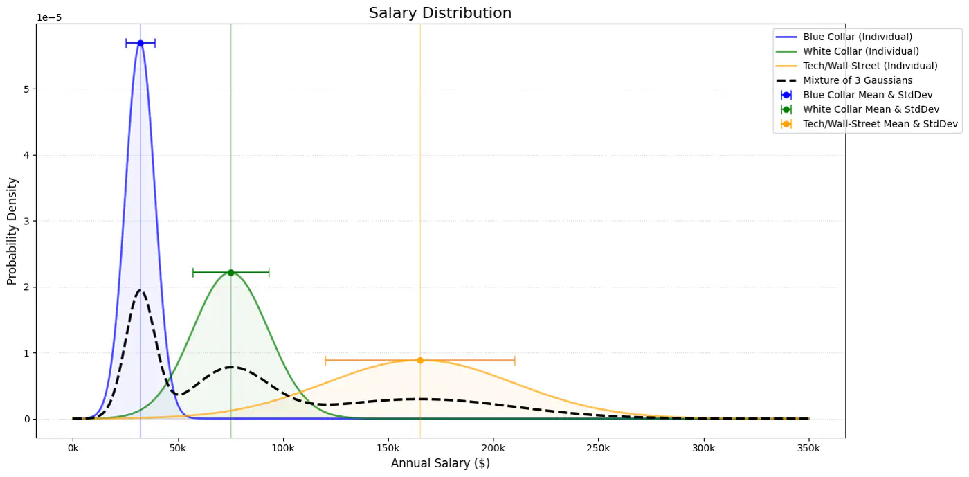
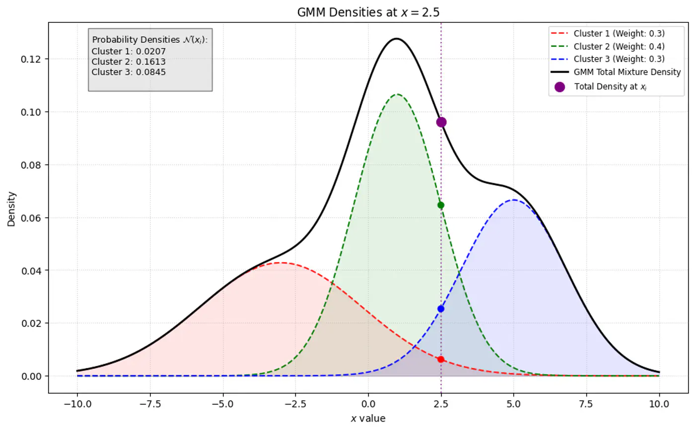
GMM represents the probability density function of the data as a weighted sum of ‘K’ component Gaussian densities.
Below plot shows the probability of a point being generated by 3 different Gaussians.
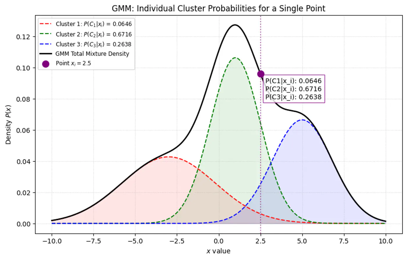
Overall density \(p(x_i|\mathbf{\theta })\) for a data point ‘\(x_i\)’:
\[p(x_i|\mathbf{\mu},\mathbf{\Sigma} )=\sum _{k=1}^{K}\pi _{k}\mathcal{N}(x_i|\mathbf{\mu }_{k},\mathbf{\Sigma }_{k})\]- K: number of component Gaussians.
- \(\pi_k\): mixing coefficient (weight) of the k-th component, such that, \(\pi_k \ge 0\) and \(\sum _{k=1}^{K}\pi _{k}=1\).
- \(\mathcal{N}(x_i|\mathbf{\mu }_{k},\mathbf{\Sigma }_{k})\): probability density function of the k-th Gaussian component with mean \(\mu_k\) and covariance matrix \(\Sigma_k\).
- \(\mathbf{\theta }=\{(\pi _{k},\mathbf{\mu }_{k},\mathbf{\Sigma }_{k})\}_{k=1}^{K}\): complete set of parameters to be estimated.
Note: \(\pi _{k}\approx \frac{\text{Number\ of\ points\ in\ cluster\ }k}{\text{Total\ number\ of\ points\ }(N)}\)
Weight of the cluster is proportional to the number of points in the cluster.
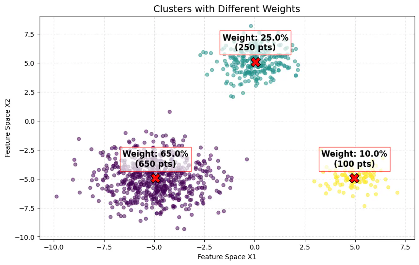
Below image shows the weighted Gaussian PDF, given the weights of clusters.
Goal of a GMM optimization is to find the set of parameters \(\Theta =\{(\pi _{k},\mu _{k},\Sigma _{k})\mid k=1,\dots ,K\}\) that maximize the likelihood of observing the given data.
\[L(\Theta |X)=\sum _{i=1}^{N}\log P(x_i|\Theta )=\sum _{i=1}^{N}\log \left(\sum _{k=1}^{K}\pi _{k}\mathcal{N}(x_i|\mu _{k},\Sigma _{k})\right)\]- \(\log (A+B)\) cannot be simplified.
- So, is there any other way ?
Imagine we are measuring the heights of people in a college.
- We see a distribution with two peaks (bimodal).
- We suspect there are two underlying groups:
- Group A (Men) and Group B (Women).
Observation:
- Observed Variable (X): Actual height measurements.
- Latent Variable (Z): The ‘label’ (Man or Woman) for each person.
Note: We did not record gender, so it is ‘hidden’ or ‘latent’.
GMM is a latent variable model, meaning each data point \(\mathbf{x}_{i}\) is assumed to have an associated unobserved (latent) variable \(z_{i}\in \{1,\dots ,K\}\) indicating which component generated it.
Note: We observe the data point, but we do not observe which cluster it belongs to (\(z_i\)).
If we knew the value of \(z_i\) (component indicator) for every point, estimating the parameters of each Gaussian component would be straightforward.
Note: The challenge lies in estimating both the parameters of the Gaussians and the values of the latent variables simultaneously.
- With ‘z’ unknown:
- maximize: \[ \log \sum _{k}\pi _{k}\mathcal{N}(x_{i}|\mu _{k},\Sigma _{k}) = \log \Big(\pi _{1}\mathcal{N}(x_{i}\mid \mu _{1},\Sigma _{1})+\pi _{2}\mathcal{N}(x_{i}\mid \mu _{2},\Sigma _{2})+ \dots + \pi _{k}\mathcal{N}(x_{i}\mid \mu _{k},\Sigma _{k})\Big)\]
- \(\log (A+B)\) cannot be simplified.
- maximize: \[ \log \sum _{k}\pi _{k}\mathcal{N}(x_{i}|\mu _{k},\Sigma _{k}) = \log \Big(\pi _{1}\mathcal{N}(x_{i}\mid \mu _{1},\Sigma _{1})+\pi _{2}\mathcal{N}(x_{i}\mid \mu _{2},\Sigma _{2})+ \dots + \pi _{k}\mathcal{N}(x_{i}\mid \mu _{k},\Sigma _{k})\Big)\]
- With ‘z’ known:
- The log-likelihood of the ‘complete data’ simplifies into a sum of logarithms:
\[\sum _{i}\log (\pi _{z_{i}}\mathcal{N}(x_{i}|\mu _{z_{i}},\Sigma _{z_{i}}))\]
- Every point is assigned to exactly one cluster, so the sum disappears because there is only one cluster responsible for that point.
- The log-likelihood of the ‘complete data’ simplifies into a sum of logarithms:
\[\sum _{i}\log (\pi _{z_{i}}\mathcal{N}(x_{i}|\mu _{z_{i}},\Sigma _{z_{i}}))\]
Note: This allows the logarithm to act directly on the exponential term of the Gaussian, leading to simple linear equations.
When ‘z’ is known, every data point is ‘labeled’ with its parent component.
To estimate the parameters (mean \(\mu_k\) and covariance \(\Sigma_k\)) for a specific component ‘k’ :
- Gather all data points \(x_i\), where \(z_i\)= k.
- Calculate the standard Maximum Likelihood Estimate.(MLE) for that single Gaussian using only those points.
Knowing ‘z’ provides exact counts and component assignments, leading to direct formulae for the parameters:
- Mean (\(\mu_k\)): Arithmetic average of all points assigned to component ‘k’.
- Covariance (\(\Sigma_k\)): Sample covariance of all points assigned to component ‘k’.
- Mixing Weight (\(\pi_k\)): Fraction of total points assigned to component ‘k’.
3 - Expectation Maximization
- If we knew the parameters (\(\mu, \Sigma, \pi\)) we could easily calculate which cluster ‘z’ each point belongs to (using probability).
- If we knew the cluster assignments ‘z’ of each point, we could easily calculate the parameters for each cluster (using simple averages).
But we do not know either of them, as the parameters of the Gaussians - we aim to find and cluster indicator latent variable is hidden.

Find latent cluster indicator variable \(z_{ik}\).
But \(z_{ik}\) is a ‘hard’ assignment’ (either ‘0’ or ‘1’).
- Because we do not observe ‘z’, we use another variable ‘Responsibility’ (\(\gamma_{ik}\)) as a ‘soft’ assignment (value between 0 and 1).
- \(\gamma_{ik}\) is the expected value of the latent variable \(z_{ik}\), given the observed data \(x_{i}\) and parameters \(\Theta\). \[\gamma _{ik}=E[z_{ik}\mid x_{i},\theta ]=P(z_{ik}=1\mid x_{i},\theta )\]
Note: \(\gamma_{ik}\) is the posterior probability (or ‘responsibility’) that cluster ‘k’ takes for explaining data point \(x_{i}\).
Using Bayes’ Theorem, we derive responsibility (posterior probability that component ‘k’ generated data point \(x_i\)) by combining the prior/weights (\(\pi_k\)) and the likelihood (\(\mathcal{N}(x_{i}\mid \mu _{k},\Sigma _{k})\)).
\[\gamma _{ik}= P(z_{ik}=1\mid x_{i},\theta ) = \frac{P(z_{ik}=1)P(x_{i}\mid z_{ik}=1)}{P(x_{i})}\]\[\gamma _{ik}=\frac{\pi _{k}\mathcal{N}(x_{i}\mid \mu _{k},\Sigma _{k})}{\sum _{j=1}^{K}\pi _{j}\mathcal{N}(x_{i}\mid \mu _{j},\Sigma _{j})}\]Bayes’ Theorem: \(P(A|B)=\frac{P(B|A)\cdot P(A)}{P(B)}\)
GMM Densities at point
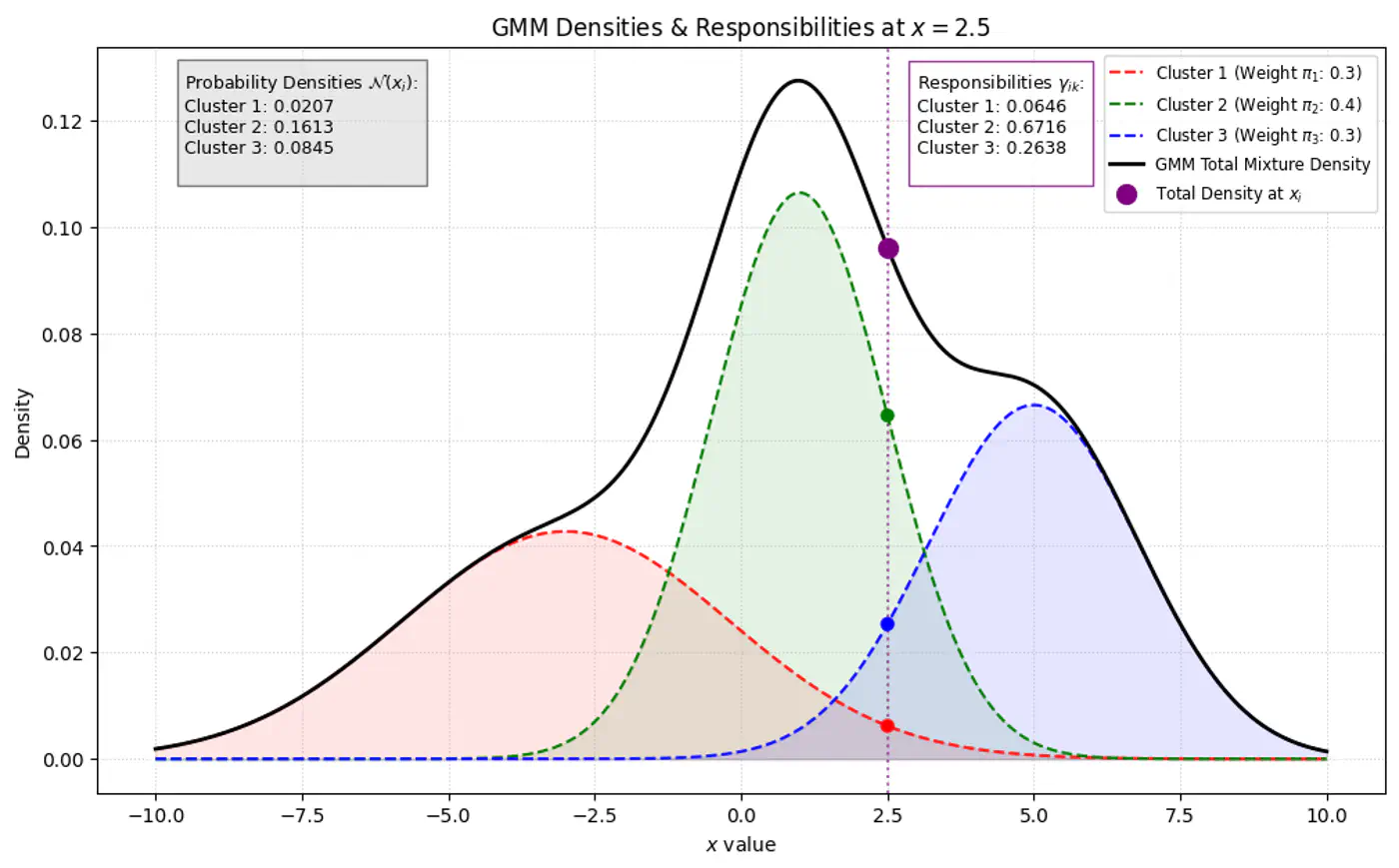
GMM Densities at point (different cluster weights)
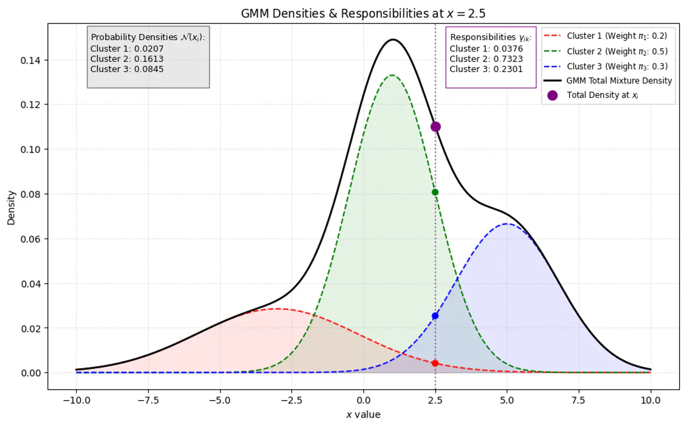
- Initialization: Assign initial values to parameters (\(\mu, \Sigma, \pi\)), often using K-Means results.
- Expectation Step (E): Calculate responsibilities; provides ‘soft’ assignments of points to clusters.
- Maximization Step (M): Update parameters using responsibilities as weights to maximize the expected log-likelihood.
- Convergence: Repeat ‘E’ and ‘M’ steps until the change in log-likelihood falls below a threshold.
Given our current guess of the clusters, what is the probability that point \(x_i\) came from cluster ‘k’ ?
\[\gamma (z_{ik})=p(z_{i}=k|\mathbf{x}_{i},\mathbf{\theta }^{(\text{old})})=\frac{\pi _{k}^{(\text{old})}\mathcal{N}(\mathbf{x}_{i}|\mathbf{\mu }_{k}^{(\text{old})},\mathbf{\Sigma }_{k}^{(\text{old})})}{\sum _{j=1}^{K}\pi _{j}^{(\text{old})}\mathcal{N}(\mathbf{x}_{i}|\mathbf{\mu }_{j}^{(\text{old})},\mathbf{\Sigma }_{j}^{(\text{old})})}\]\(\pi_k\) : Probability that a randomly selected data point \(x_i\) belongs to the k-th component before we even look at the specific value of \(x_i\), such that \(\pi_k \ge 0\) and \(\sum _{k=1}^{K}\pi _{k}=1\).
Update the parameters (\(\mu, \Sigma, \pi\)) by calculating weighted versions of the standard MLE formulas using responsibilities as weight ️♀️.
\[ \begin{align*} &\bullet \mathbf{\mu }_{k}^{(\text{new})}=\frac{1}{N_{k}}\sum _{i=1}^{N}\gamma (z_{ik})\mathbf{x}_{i} \\ &\bullet \mathbf{\Sigma }_{k}^{(\text{new})}=\frac{1}{N_{k}}\sum _{i=1}^{N}\gamma (z_{ik})(\mathbf{x}_{i}-\mathbf{\mu }_{k}^{(\text{new})})(\mathbf{x}_{i}-\mathbf{\mu }_{k}^{(\text{new})})^{\top } \\ &\bullet \pi _{k}^{(\text{new})}=\frac{N_{k}}{N} \end{align*} \]- where, \(N_{k}=\sum _{i=1}^{N}\gamma (z_{ik})\) is the effective number of points assigned to component ‘k'.