This is the multi-page printable view of this section. Click here to print.
K Means
1 - K Means
🌍In real-world systems, labeled data is scarce and expensive 💰.
💡Unsupervised learning discovers inherent structure without human annotation.
👉Clustering answers: “Given a set of points, what natural groupings exist?”
- Customer Segmentation: Group users by behavior without predefined categories.
- Image Compression: Reduce color palette by clustering pixel colors.
- Anomaly Detection: Points far from any cluster are outliers.
- Data Exploration: Understand structure before building supervised models.
- Preprocessing: Create features from cluster assignments.
💡Clustering assumes that ‘similar’ points should be grouped together.
👉But what is ‘similar’? This assumption drives everything.
Given:
- Dataset X = {x₁, x₂, …, xₙ} where xᵢ ∈ ℝᵈ.
- Desired number of clusters ‘k'.
Find:
Cluster assignments C = {C₁, C₂, …, Cₖ}.
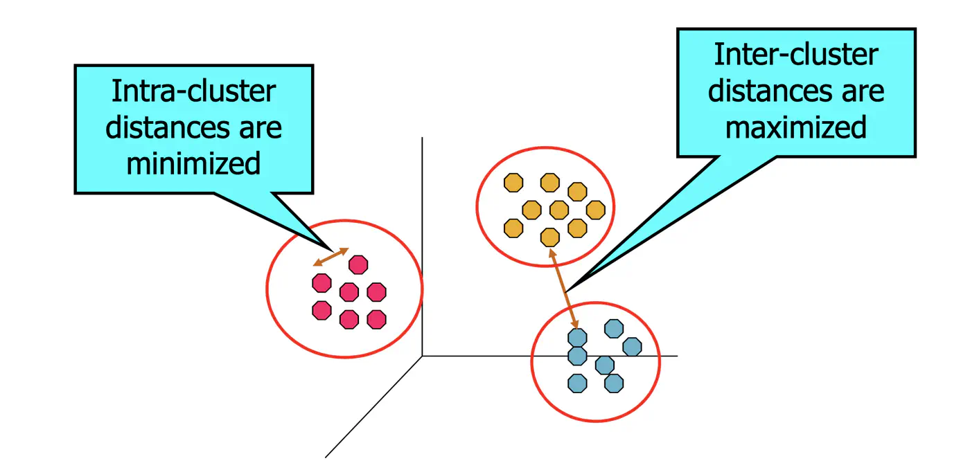
Such that points within clusters are ‘similar’.
And points across clusters are ‘dissimilar’.
This is fundamentally an optimization problem, i.e, find parameters such that the value is minimum/maximum. We need:
- An objective function
- what makes a clustering ‘good’?
- An algorithm to optimize it
- how do we find good clusters?
- Evaluation metrics
- how do we measure quality?
Objective function:
👉Minimize the within-cluster sum of squares (WCSS).
- Where:
- C = {C₁, …, Cₖ} are cluster assignments.
- μⱼ is the centroid (mean) of cluster Cₖ.
- ||·||² is squared Euclidean distance.
Note: Every point belongs to one and only one cluster.
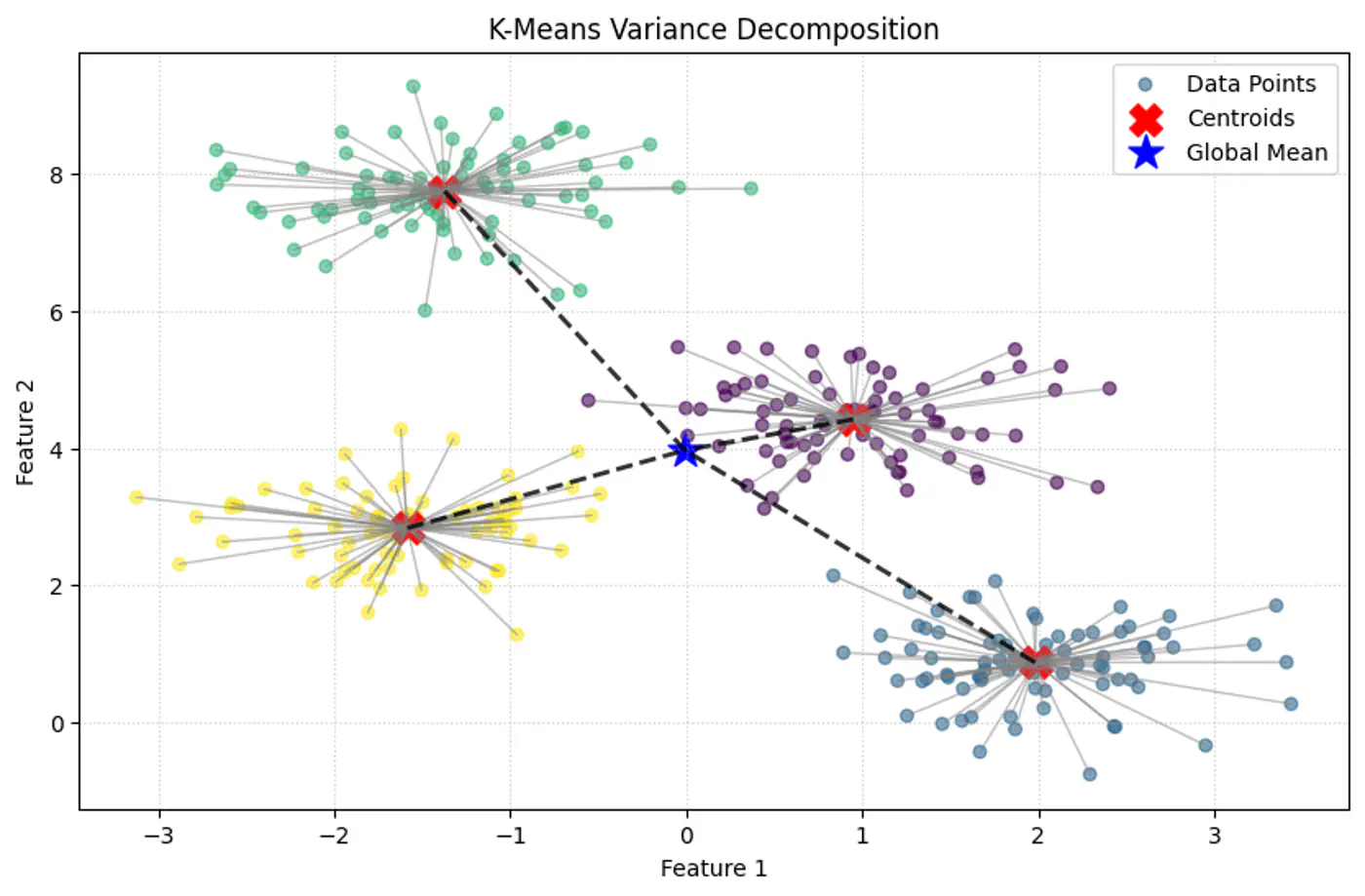
💡Within-Cluster Sum of Squares (WCSS) is nothing but variance.
⭐️ Total Variance = Within-Cluster Variance + Between-Cluster Variance
👉K-Means minimizes within-Cluster variance, which implicitly maximizes between-cluster separation.
Geometric Interpretation:
- Each point is ‘pulled’ toward its cluster center.
- The objective measures total squared distance of all points to their centers.
- Lower J(C, μ) means tighter, more compact clusters.
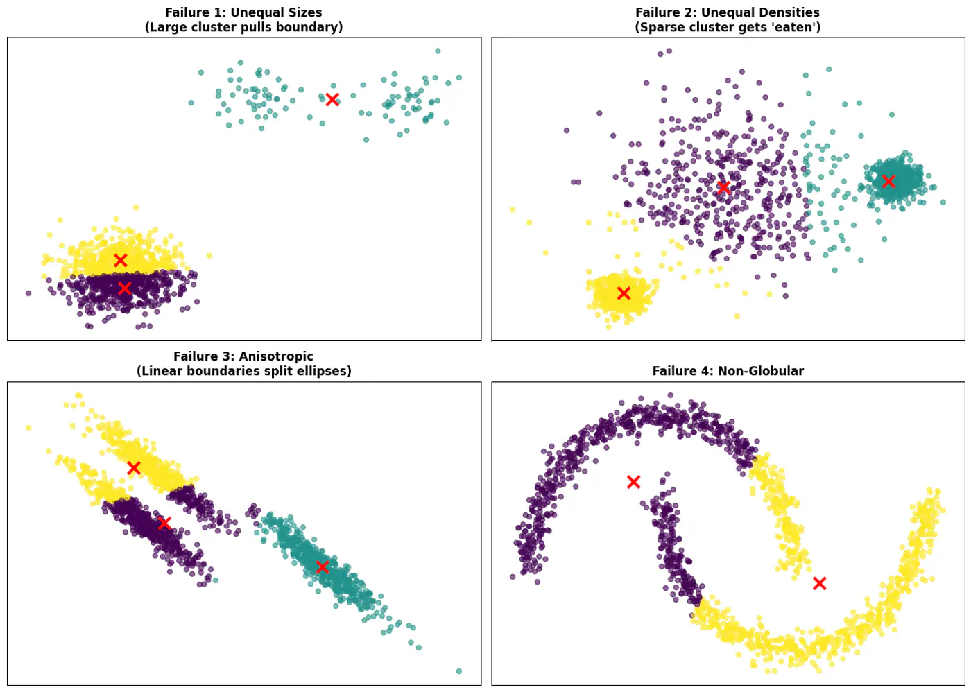
Note: K-Means works best when clusters are roughly spherical, similarly sized, and well-separated.
⭐️The problem requires partitioning ’n’ observations into ‘k’ distinct, non-overlapping clusters, which is given by the Stirling number of the second kind, which grows at a rate roughly equal to \(k^n/k!\).
\[S(n,k)=\frac{1}{k!}\sum _{j=0}^{k}(-1)^{k-j}{k \choose j}j^{n}\]\[S(100,2)=2^{100-1}-1=2^{99}-1\]\[2^{99}\approx 6.338\times 10^{29}\]👉This large number of possible combinations makes the problem NP-Hard.
🦉The k-means optimization problem is NP-hard because it belongs to a class of problems for which no efficient (polynomial-time ⏰) algorithm is known to exist.
End of Section
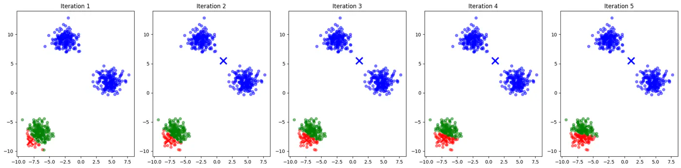
2 - Lloyds Algorithm
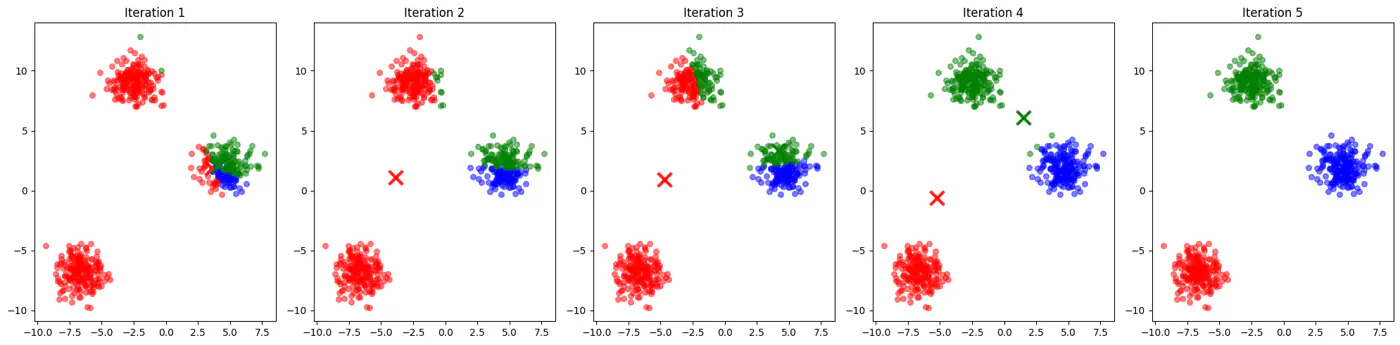
Iterative method for partitioning ’n’ data points into ‘k’ groups by repeatedly assigning data points to the nearest centroid (mean) and then recalculating centroids until assignments stabilize, aiming to minimize within-cluster variance.
📥Input: X = {x₁, …, xₙ}, ‘k’ (number of clusters)
📤Output: ‘C’ (clusters), ‘μ’ (centroids)
👉Steps:
- Initialize: Randomly choose ‘k’ cluster centroids μ₁, …, μₖ.
- Repeat until convergence, i.e, until cluster assignments and centroids no longer change significantly.
- a) Assignment: Assign each data point to the cluster whose centroid is closest (usually using Euclidean distance).
- For each point xᵢ: cᵢ = argminⱼ ||xᵢ - μⱼ||²
- b) Update: Recalculate the centroid (mean) of each cluster.
- For each cluster j: μⱼ = (1/|Cⱼ|) Σₓᵢ∈Cⱼ xᵢ
- Initialization sensitive, different initialization may lead to different clusters.
- Tries to make each cluster of same size that may not be the case in real world.
- Tries to make each cluster with same density(variance)
- Does not work well with non-globular(spherical) data.
👉See how 2 different runs of K-Means algorithm gives totally different clusters.

👉Also, K-Means does not work well with non-spherical clusters, or clusters with different densities and sizes.
✅ Do not select initial points randomly, but some logic, such as, K-means++ algorithm.
✅ Use hierarchical clustering or density based clustering DBSCAN.
End of Section
3 - K Means++
- If two initial centroids belong to the same natural cluster, the algorithm will likely split that natural cluster in half and be forced to merge two other distinct clusters elsewhere to compensate.
- Inconsistent; different runs may lead to different clusters.
- Slow convergence; Centroids may need to travel much farther across the feature space, requiring more iterations.
👉Example for different K-Means algorithm runs give different clusters

💡Addresses the issue due to random initialization by aiming to spread out the initial centroids across the data points.
Steps:
- Select the first centroid: Choose one data point randomly from the dataset to be the first centroid.
- Calculate distances: For every data point x not yet selected as a centroid, calculate the distance, D(x), between x and the nearest centroid chosen so far.
- Select the next centroid: Choose the next centroid from the remaining data points with a probability
proportional to D(x)^2.
This makes it more likely that a point far from existing centroids is selected, ensuring the initial centroids are well-dispersed. - Repeat: Repeat steps 2 and 3 until ‘k’ number of centroids are selected.
- Run standard K-means: Once the initial centroids are chosen, the standard k-means algorithm proceeds with assigning data points to the nearest centroid and iteratively updating the centroids until convergence.
End of Section
4 - K Medoid
- In K-Means, the centroid is the arithmetic mean of the cluster. The mean is very sensitive to outliers.
- Not interpretable; centroid is the mean of cluster data points and may not be an actual data point, hence not representative.
⭐️Medoid is a specific data point from a dataset that acts as the ‘center’ or most representative member of its cluster.
👉It is defined as the object within a cluster whose average dissimilarity (distance) to all other members in that same cluster is the smallest.
💡Selects actual data points from the dataset as cluster representatives, called medoids (most centrally located).
👉a.k.a Partitioning Around Medoids(PAM).
Steps:
- Initialization: Select ‘k’ data points from the dataset as the initial medoids using K-Means++ algorithm.
- Assignment: Calculate the distance (e.g., Euclidean or Manhattan) from each non-medoid point to all medoids and assign each point to the cluster of its nearest medoid.
- Update (Swap):
- For each cluster, swap current medoid with a non-medoid point from the same cluster.
- For each swap, calculate the total cost 💰(sum of distances from medoid).
- Pick the medoid with minimum cost 💰.
- Repeat🔁: Repeat the assignment and update steps until (convergence), i.e, medoids no longer change or a maximum number of iterations is reached.
Note: Kind of brute-force algorithm, computationally expensive for large dataset.
✅ Flexible Distance Metrics: It can work with any dissimilarity measure (Manhattan, Cosine similarity), making it ideal for categorical or non-Euclidean data.
✅ Interpretable Results: Cluster centers are real observations (e.g., a ‘typical’ customer profile), which makes the output easier to explain to stakeholders.
End of Section
5 - Clustering Quality Metrics
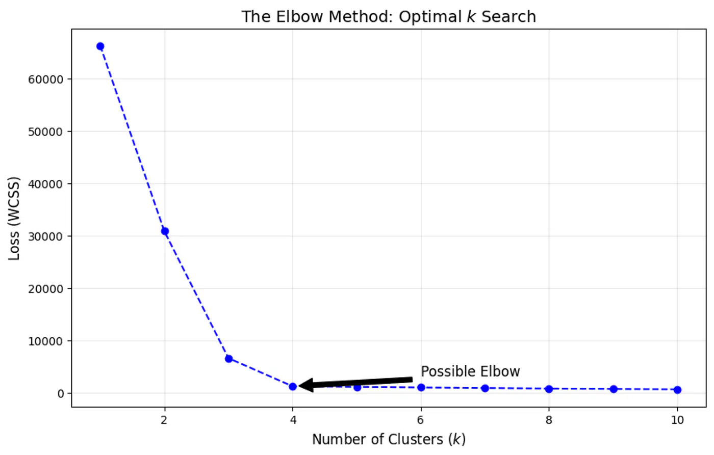
- 👉 Elbow Method: Quickest to compute; good for initial EDA (Exploratory Data Analysis).
- 👉 Dunn Index: Focuses on the ‘gap’ between the closest clusters.
- 👉 Silhouette Score: Balances compactness and separation.
- 👉 Domain specific knowledge and system constraints.
⭐️Heuristic used to determine the optimal number of clusters (k) for clustering by visualizing how the quality of clustering improves as ‘k’ increases.
🎯The goal is to find a value of ‘k’ where adding more clusters provides a diminishing return in terms of variance reduction.
⭐️Clustering quality evaluation metric that measures: separation (between clusters) and compactness (within clusters)
Note: A higher Dunn Index value indicates better clustering, meaning clusters are well-separated from each other and compact.
👉Dunn Index Formula:
\[DI = \frac{\text{Minimum Inter-Cluster Distance(between different clusters)}}{\text{Maximum Intra-Cluster Distance(within a cluster)}}\]\[DI = \frac{\min_{1 \le i < j \le k} \delta(C_i, C_j)}{\max_{1 \le l \le k} \Delta(C_l)}\]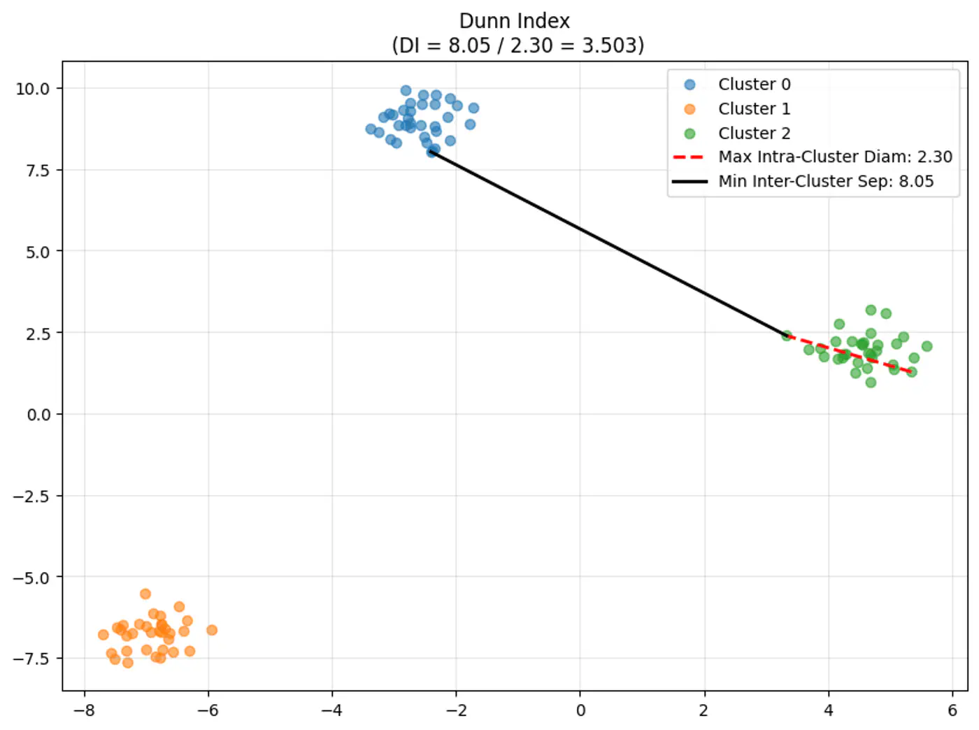
👉Let’s understand the terms in the above formula:
\(\delta(C_i, C_j)\) (Inter-Cluster Distance):
- Measures how ‘far apart’ the clusters are.
- Distance between the two closest points of different clusters (Single-Linkage distance). \[\delta(C_i, C_j) = \min_{x \in C_i, y \in C_j} d(x, y)\]
\(\Delta(C_l)\) (Intra-Cluster Diameter):
- Measures how ‘spread out’ a cluster is.
- Distance between the two furthest points within the same cluster (Complete-Linkage distance). \[\Delta(C_l) = \max_{x, y \in C_l} d(x, y)\]
- Single Linkage (MIN): Uses the minimum distance between any two points in different clusters.
- Complete Linkage (MAX): Uses the maximum distance between any two points in same cluster.
End of Section
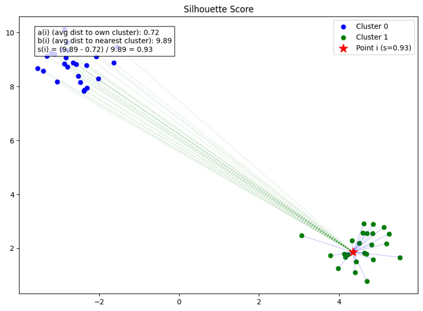
6 - Silhouette Score
- ✅ Elbow Method: Quickest to compute; good for initial EDA.
- ✅ Dunn Index: Focuses on the ‘gap’ between the closest clusters.
——- We have seen the above 2 methods in the previous section ———- - 👉 Silhouette Score: Balances compactness and separation.
- 👉 Domain specific knowledge and system constraints.
⭐️Clustering quality evaluation metric that measures how similar a data point is to its own cluster (cohesion) compared to other clusters (separation).
Note: Higher scores (closer to 1) indicate better-defined, distinct clusters, while scores near 0 suggest overlapping clusters, and negative scores mean points might be in the wrong cluster.
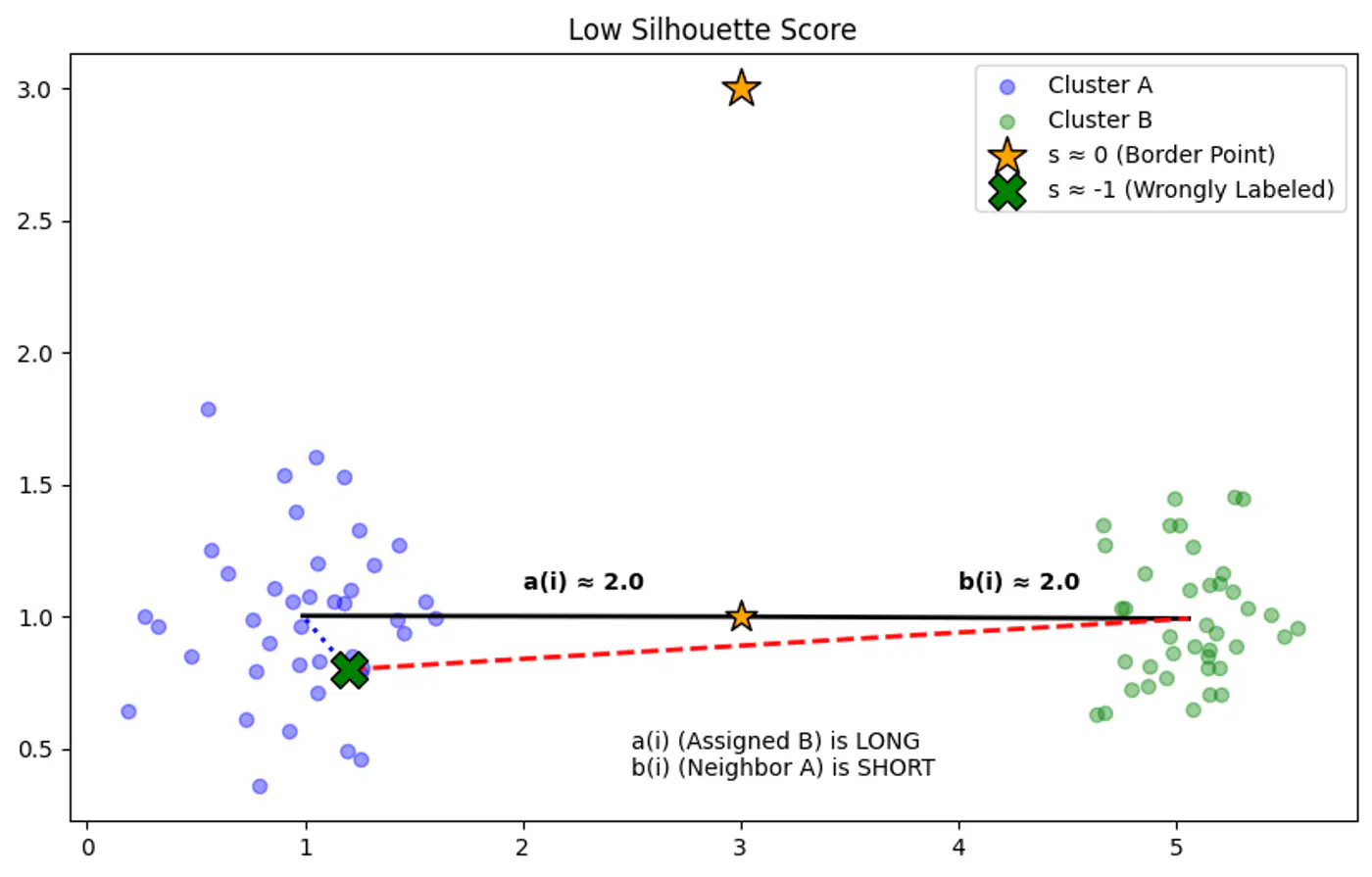
Silhouette score for point ‘i’ is the difference between separation b(i) and cohesion a(i), normalized by the larger of the two.
\[ s(i) = \frac{b(i) - a(i)}{\max(a(i), b(i))} \]Note: The Global Silhouette Score is simply the mean of s(i) for all points in the dataset.
👉Example for Silhouette Score:
👉Example for Silhouette Score of 0(Border Point) and negative(Wrong Cluster).
🦉Now let’s understand the terms in Silhouette Score in detail.
Average distance between point ‘i’ and all other points in the same cluster.
\[a(i) = \frac{1}{|C_A| - 1} \sum_{j \in C_A, i \neq j} d(i, j)\]Note: Lower a(i) means the point is well-matched to its own cluster.
Average distance between point ‘i’ and all points in the nearest neighboring cluster (the cluster that ‘i’ is not a part of, but is closest to).
\[b(i) = \min_{C_B \neq C_A} \frac{1}{|C_B|} \sum_{j \in C_B} d(i, j)\]Note: Higher b(i) means the point is very far from the next closest cluster.
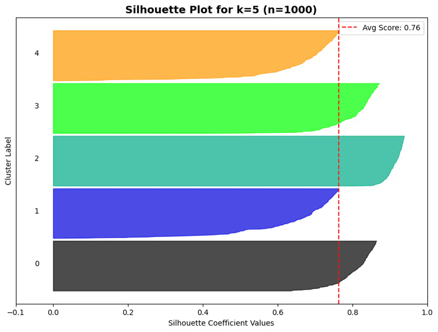
⭐️A silhouette plot is a graphical tool used to evaluate the quality of clustering algorithms (like K-Means), showing how well each data point fits within its cluster.
👉Each bar gives the average silhouette score of the points assigned to that cluster.
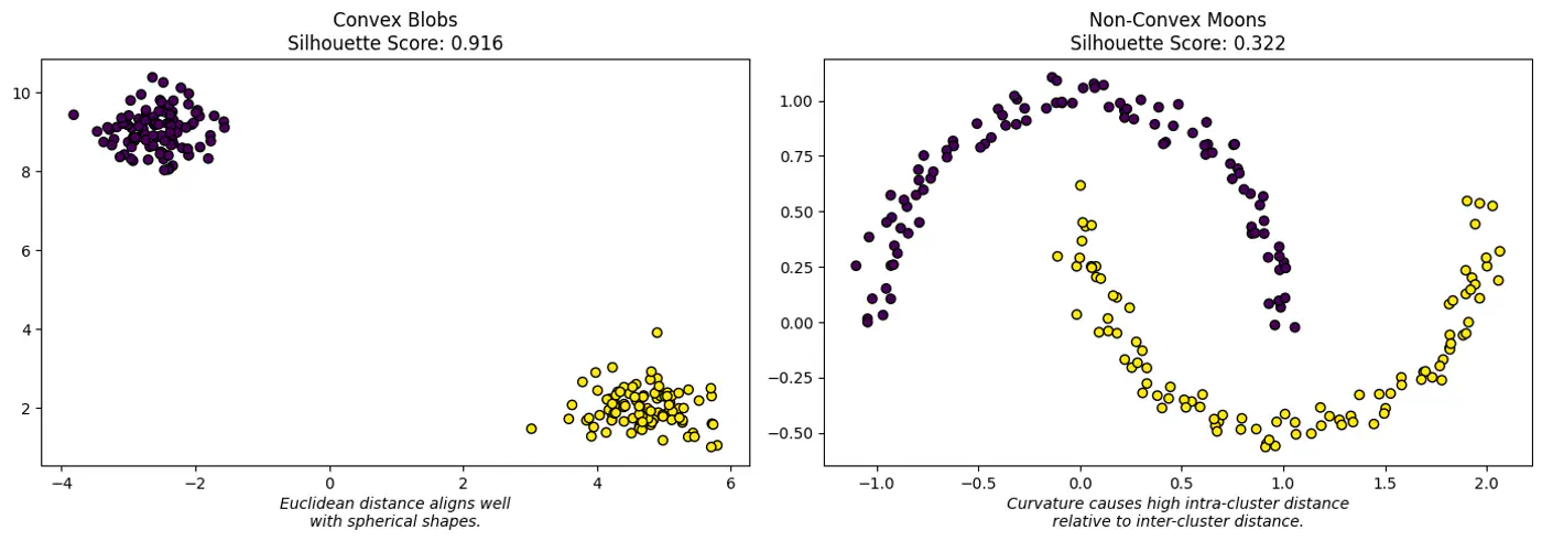
⛳️ Like K-Means, the Silhouette Score (when using Euclidean distance) assumes convex clusters.
🌘 If we use it on ‘Moon’ shaped clusters, it will give a low score even if the clusters are perfectly separated, because the ‘average distance’ to a neighbor might be small due to the curvature of the manifold.
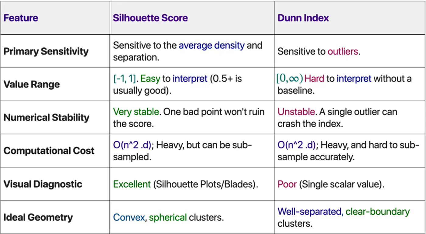
Choose Silhouette Score if:
✅ Need a human-interpretable metric to present to stakeholders.
✅ Dealing with real-world noise and overlapping ‘fuzzy’ boundaries.
✅ Want to see which specific clusters are weak (using the plot).
Choose Dunn Index if:
✅ Performing ‘Hard Clustering’ where separation is a safety or business requirement.
✅ Data is pre-cleaned of outliers (e.g., in a curated embedding space).
✅ Need to compare different clustering algorithms (e.g., K-Means vs. DBSCAN) on a high-integrity task.
End of Section