This is the multi-page printable view of this section. Click here to print.
Maths
- 1: Probability
- 1.1: Introduction to Probability
- 1.2: Conditional Probability
- 1.3: Independence of Events
- 1.4: Cumulative Distribution Function
- 1.5: Probability Mass Function
- 1.6: Probability Density Function
- 1.7: Expectation
- 1.8: Moment Generating Function
- 1.9: Joint & Marginal
- 1.10: Independent & Identically Distributed
- 1.11: Convergence
- 1.12: Law of Large Numbers
- 1.13: Markov's Inequality
- 1.14: Cross Entropy & KL Divergence
- 1.15: Parametric Model Estimation
- 2: Statistics
- 2.1: Data Distribution
- 2.2: Correlation
- 2.3: Central Limit Theorem
- 2.4: Confidence Interval
- 2.5: Hypothesis Testing
- 2.6: T-Test
- 2.7: Z-Test
- 2.8: Chi-Square Test
- 2.9: Performance Metrics
- 3: Linear Algebra
- 3.1: Vector Fundamentals
- 3.2: Matrix Operations
- 3.3: Eigen Value Decomposition
- 3.4: Singular Value Decomposition
- 3.5: Principal Component Analysis
- 3.6: Vector & Matrix Calculus
- 3.7: Vector Norms
- 3.8: Hyperplane
- 4: Calculus
- 4.1: Calculus Fundamentals
- 4.2: Optimization
- 4.3: Gradient Descent
- 4.4: Newton's Method
1.1 - Introduction to Probability
Because the world around us is very uncertain, and Probability acts as -
the fundamental language
to understand, express and deal with this uncertainty.
- Toss a fair coin, \(P(H) = P(T) = 1/2\)
- Roll a die, \(P(1) = P(2) = P(3) = P(4) = P(5) = P(6) = 1/6\)
- Email classifier, \(P(spam) = 0.95 ,~ P(not ~ spam) = 0.05\)
Range: \([0,1]\)
\(P=0\): Highly unlikely
\(P=1\): Almost certain
Symbol: \(\Omega\)
\(P(\Omega) = 1\)
- Toss a fair coin, sample space: \(\Omega = \{H,T\}\)
- Roll a die, sample space: \(\Omega = \{1,2,3,4,5,6\}\)
- Choose a real number \(x\) from the interval \([2,3]\), sample space: \(\Omega = [2,3]\); sample size = \(\infin\)
Note: There can be infinitely many points between 2 and 3, e.g: 2.21, 2.211, 2.2111, 2.21111, … - Randomly put a point in a rectangular region; sample size = \(\infin\)
Note: There can be infinitely many points in any rectangular region.
A,B,…⊆Ω
- Toss a fair coin, set of possible outcomes: \(\{H,T\}\)
- Roll a die, set of possible outcomes: \(\{1,2,3,4,5,6\}\)
- Roll a die, event \(A = \{1,2\} => P(A) = 2/6 = 1/3\)
- Email classifier, set of possible outcomes: \(\{spam,not ~spam\}\).
- Toss a fair coin, possible outcomes: \(\Omega = \{H,T\}\)
- Roll a die, possible outcomes: \(\Omega = \{1,2,3,4,5,6\}\)
- Choose a real number \(x\) from the interval \([2,3]\) with decimal precision, sample space: \(\Omega = [2,3]\).
Note: There are 99 real numbers between 2 and 3 with 2 decimal precision i.e from 2.01 to 2.99. - Number of cars passing a specific traffic signal in 1 hour.
- A line segment between 2 and 3 - forms a continuum.
- Randomly put a point in a rectangular region.
graph TD
    A[Sample Space] --> |Discrete| B(Finite)
    A --> C(Infinite)
    C --> |Discrete| D(Countable)
C --> |Continuous| E(Uncountable)No overlapping or common outcomes.
If one event occurs, then the other event does NOT occur.
- Roll a die, sample space: \(\Omega = \{1,2,3,4,5,6\}\)
Odd outcome = \(A = \{1,3,5\}\)
Even outcome = \(B = \{2,4,6\}\) are mutually exclusive.
\(P(A \cap B) = 0\)
Since, \(P(A \cup B) = P(A) + P(B) - (P(A \cap B)\)
Therefore, \(P(A \cup B) = P(A) + P(B)\)
Note: If we know that event \(A\) has occurred, then we can say for sure that the event \(B\) did NOT occur.
- Roll a die twice , sample space: \(\Omega = \{1,2,3,4,5,6\}\)
Odd number in 1st throw = \(A = \{1,3,5\}\)
Odd number in 2nd throw = \(B = \{1,3,5\}\)
Note: A and B are independent because whether we get an odd number in 1st roll has NO impact of getting an odd number in second roll.
\(P(A \cap B) = P(A)*P(B)\)
Note: If we know that event \(A\) has occurred, then that gives us NO new information about the event \(B\).
Let’s understand this answer with an example.
Probability of choosing exactly one point on the number line or a real number, say 2.5,
from the interval \([2,3]\) is almost = 0, because there are infinitely many points between 2 and 3.
Also, we can NOT say that choosing exactly 2.5 is impossible, because it exists there on the number line.
But, for all practical purposes, \(P(2.5) = 0\).
Therefore, we say that \(P=0\) means “Highly Unlikely” and NOT “Impossible”.
Extending this line of reasoning, we can say that probability of NOT choosing 2.5, \(P(!2.5) = 1\).
Theoretically yes, because there are infinitely many points between 2 and 3.
But, we cannot say for sure that we cannot choose 2.5 exactly.
There is some probability of choosing 2.5, but it is very small.
Therefore, we say that \(P=1\) means “Almost Sure” and NOT “Certain”.
Here, in this case we can say that \(P(7)=0\) and that means Impossible.
Similarly, we can say that \(P(get ~any ~number ~between ~1 ~and ~6)=1\) and \(P=1 => \) Certain.
End of Section
1.2 - Conditional Probability
It is the probability of an event occurring, given that another event has already occurred.
Allows us to update probability when additional information is revealed.
\(P(A \cap B) = P(A)*P(B \mid A)\)
- Roll a die, sample space: \(\Omega = \{1,2,3,4,5,6\}\)
Event A = Get a 5 = \(\{5\} => P(A) = 1/6\)
Event B = Get an odd number = \(\{1, 3, 5\} => P(B) = 3/6 = 1/2\)
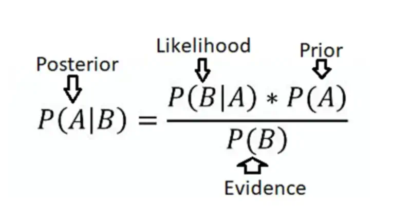
It is a formula that uses conditional probability.
It allows us to update our belief about an event’s probability based on new evidence.
We know from conditional probability and chain rule that:
Combining all the above equations gives us the Bayes’ Theorem:
$$ \begin{aligned} P(A \mid B) = \frac{P(A)*P(B \mid A)}{P(B)} \end{aligned} $$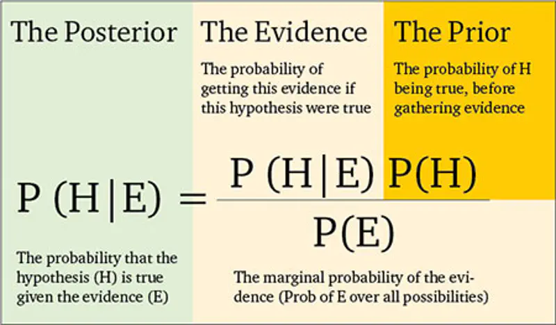
- Roll a die, sample space: \(\Omega = \{1,2,3,4,5,6\}\)
Event A = Get a 5 = \(\{5\} => P(A) = 1/6\)
Event B = Get an odd number = \(\{1, 3, 5\} => P(B) = 3/6 = 1/2\)
Task: Find the probability of getting a 5 given that you rolled an odd number.
\(P(B \mid A) = 1\) = Probability of getting an odd number given that we have rolled a 5.
Now, let’s understand another concept called Law of Total Probability.
Here, we can say that the sample space \(\Omega\) is divided into 2 parts - \(A\) and \(A ^ \complement \)
So, the probability of an event \(B\) is given by:
\[ B = B \cap A + B \cap A ^ \complement \\ P(B) = P(B \cap A) + P(B \cap A ^ \complement ) \\ By ~Chain ~Rule: P(B) = P(A)*P(B \mid A) + P(A ^ \complement )*P(B \mid A ^ \complement ) \]Overall probability of an event B, considering all the different, mutually exclusive ways it can occur.
If A₁, A₂, …, Aₙ are a set of events that partition the sample space, such that they are -
- Mututally exclusive : \(A_i \cap A_j = \emptyset\) for all \(i, j\)
- Exhaustive: \(A₁ \cup A₂ ... \cup Aₙ = \Omega\) for all \(i \neq j\) \[ P(B) = \sum_{i=1}^{n} P(A_i)*P(B \mid A_i) \] where \(n\) is the number of mutually exclusive partitions of the sample space \(\Omega\) .
End of Section
1.3 - Independence of Events
Two events are independent if the occurrence of one event does not affect the probability of the other event.
There are 3 types of independence of events:
- Mutual Independence
- Pair-Wise Independence
- Conditional Independence
Joint probability of two events is equal to the product of the individual probabilities of the two events.
\(P(A \cap B) = P(A)*P(B)\)
Joint probability: The probability of two or more events occurring simultaneously.
\(P(A \cap B)\) or \(P(A, B)\)
- Toss a coin and roll a die -
\(A\) = Get a heads; \(P(A)=1/2\)
\(B\) = Get an odd number; \(P(B)=1/2\)
=> A and B are mutually independent.
Pair-wise independence != Mutual independence.
- Toss 3 coins;
For 2 tosses, sample space: \(\Omega = \{HH,HT, TH, TT\}\)
\(A\) = First and Second toss outcomes are same i.e \(\{HH, TT\}\); \(P(A)= 2/4 = 1/2\)
\(B\) = Second and Third toss outcomes are same i.e \(\{HH, TT\}\); \(P(B)= 2/4 = 1/2\)
\(C\) = Third and First toss outcomes are same i.e \(\{HH, TT\}\); \(P(C)= 2/4 = 1/2\)
Now, pair-wise independence of the above events A & B is - \(P(A \cap B)\)
\(P(A \cap B)\) => Outcomes of first and second toss are same &
outcomes of second and third toss are same.
=> Outcomes of all the three tosses are same.
Total number of outcomes = 8
Desired outcomes = \(\{HHH, TTT\}\) = 2
=> \(P(A \cap B) = 2/8 = 1/4 = P(A) * P(B) = 1/2 * 1/2 = 1/4\)
Therefore, \(A\) and \(B\) are pair-wise independent.
Similarly, we can also prove that \(A\) and \(C\) and \(B\) and \(C\) are also pair-wise independent.
Now, let’s check for mutual independence of the above events A, B & C.
\(P(A \cap B \cap C) = P(A)*P(B)*P(C)\)
\(P(A \cap B \cap C)\) = Outcomes of all the three tosses are same i.e \(\{HHH, TTT\}\)
Total number of outcomes = 8
Desired outcomes = \(\{HHH, TTT\}\) = 2
So, \(P(A \cap B \cap C)\) = 2/8 = 1/4
But, \(P(A)*P(B)*P(C) = 1/2*1/2*1/2 = 1/8\)
Therefore \(P(A \cap B \cap C)\) ≠ \(P(A)*P(B)*P(C)\)
=> \(A, B, C\) are NOT mutually independent but only pair wise independent.
if they are independent given that C has occurred.
Occurrence of C changes the context, causing the events A & B to become independent of each other.
=> A & B are NOT independent.
Now, let’s check for conditional independence of A & B given C.
Therefore, A & B are conditionally independent given C.
End of Section
1.4 - Cumulative Distribution Function
Random Variable X is represented as, \(X: \Omega \to \mathbb{R} \)
👉 It maps abstract outcomes of a random experiment to concrete numerical values required for mathematical analysis.
- Toss a coin 2 times, sample space: \(\Omega = \{HH,HT, TH, TT\}\)
The above random experiment of coin tosses can be mapped to a random variable \(X: \Omega \to \mathbb{R} \)
\(X: \Omega = \{HH,HT, TH, TT\} \to \mathbb{R}) \)
Say, if we count the number of heads, then
\[ \begin{aligned} X(0) = \{TT\} = 1 \\ X(1) = \{HT, TH\} = 2 \\ X(2) = \{HH\} = 1 \\ \end{aligned} \] Similar, output will be observed for number of tails.
Depending upon the nature of output, random variables are of 2 types - Discrete and Continuous.
Typically obtained by counting.
Discrete random variable cannot take any value between 2 consecutive values.
Possible outcomes are infinite.
- A person’s height in a given range of say 150cm-200cm.
Height can take any value, not just round values, e.g: 150.1cm, 167.95cm, 180.123cm etc.
Now, that we have understood that how random variable can be used to map outcomes of abstract random experiment to real values for mathematical analysis, we will understand its applications.
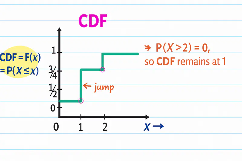
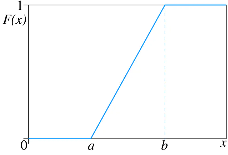
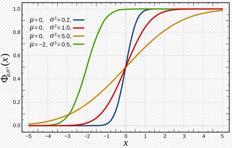
CDF = \(F(X) = P(X \leq x)\) i.e Probability a random variable \(X\) will take for a value \(<=x\).
- Discrete random variable - Toss a coin 2 times, sample space: \(\Omega = \{HH,HT, TH, TT\}\)
Count the number of heads.
\[ \begin{aligned} X(0) = \{TT\} = 1 => P(X = 0) = 1/4 \\ X(1) = \{HT, TH\} = 2 => P(X = 1) = 1/2\\ X(2) = \{HH\} = 1 => P(X = 2) = 1/4 \\ \\ CDF = F(X) = P(X \leq x) \\ F(0) = P(X \leq 0) = P(X < 0) + P(X = 0) = 1/4 \\ F(1) = P(X \leq 1) = P(X < 1) + P(X = 1) = 1/4 + 1/2 = 3/4 \\ F(2) = P(X \leq 2) = P(X < 2) + P(X = 2) = 3/4 + 1/4 = 1 \\ \end{aligned} \]
- Continuous random variable - Consider a line segment/interval from \(\Omega = [0,2] \)
Random variable \(X(\omega) = \omega\)
i.e \(X(1) = 1 ~and~ X(1.1) = 1.1 \)
\[ \begin{aligned} P[(0,1/2)] = (1/2)/2 = 1/4 \\ P[(3/4, 2)] = (2-3/4)/2 = 5/8 \\ P(X<=1.1) = P(-\infty, 1.1)/2 = 1.1/2 \end{aligned} \] \[ F_X(x) = P(X \leq x) = \begin{cases} \frac{x}{2} & \text{if } x \in [0,2] \\ 1 & \text{if } x > 2 \\ 0 & \text{if } x < 0 \end{cases} \]
- Non-Decreasing:
For any 2 values \(x_1\) and \(x_2\) such that \(x_1 \leq x_2\), corresponding CDF must satisfy -
\(F(x_1) \leq F(x_2)\)
Note: Cumulative function can never decrease as x increases. - Bounded:
Range of CDF is always between 0 and 1, because CDF represents total probability, which cannot be negative or greater than 1.
\(\lim_{x \to -\infty} F(X) = 0\); as \(x \to -\infty\), event \((X \le x)\) becomes an impossible event
i.e \(P(X \le x) =0\)
\(\lim_{x \to \infty} F(X) = 1\); as \(x \to \infty\), event \((X \le x)\) includes all possible outcomes of the event, making sure that \(P(X \le x) =1\) - Right Continuous:
Function’s value at a point is same as the limit of the function, as we approach that point from right hand side (RHS).
Note: Reason for only right continuity is because how the cumulative distribution function is defined, as we may have a jump on the left side of the point.
\(\lim_{h \to o^+} F(X+h) = F(X)\)
For example:
In the above coin toss CDF example, if we approach X=1 from right, say 1.001, 1.01 etc, the value of \(F(X) = P(X \leq x) = F(1) = 3/4\).
But, if we approach \(X=1\) from left, say 0.99, 0.999 etc, the value of \(F(X) = 1/4\), as these values do NOT yet include the value of the probability at \(X=1\).
Value of the probability of a random variable X, at any given value x, is calculated by summing up all the probabilities for values \(\le x\).
\( CDF = F_X(x) = \sum_{x_i \le x} P(X=x_i) \), where \(P(X=x_i)\) is the Probability Mass Function (PMF) at \(x_i\)
In the above coin toss example -
Height of the jump at ‘x’ = Probability at that value ‘x’.
e.g: Jump at (x=1) = 1/2 = Probability at (x=1).
CDF for continuous random variable is calculated by integrating the probability density function (PDF) from \(-\infty\) to the given value \(x\).
\( CDF = F_X(x) = \int_{-\infty}^{x} f(x) \,dx \), where \(f(x)\) is the Probability Density Function (PDF) of random variable.
Note: We can also say that PDF is the derivative of CDF for continuous random variable.
\(PDF = f(x) = F'(X) = \frac{dF_X(x)}{dx} \)
Read more about Integration
End of Section
1.5 - Probability Mass Function
It assigns a “non-zero” mass or probability to a specific countable outcome.
Note: Called ‘mass’ because probability is concentrated at a single discrete point.
\(PMF = P(X=x)\)
e.g: Bernoulli, Binomial, Multinomial, Poisson etc.
Commonly visualised as a bar chart.
Note: PMF = Jump at a given point in CDF.
\(PMF = P_x(X=x_i) = F_X(X=x_i) - F_X(X=x_{i-1})\)
- Non-Negative: Probability of any value ‘x’ must be non-negative i.e \(P(X=x) \ge 0 ~\forall x~\).
- Sum = 1: Sum of probabilities of all possible outcomes must be 1.
\( \sum_{x} P(X=x) = 1 \) - For any value that the discrete random variable can NOT take, the probability must be zero.
p = Probability of success
1-p = Probability of failure
Mean = p
Variance = p(1-p)
Note: A single trial that adheres to these conditions is called a Bernoulli trial.
\(PMF, P(x) = p^x(1-p)^{1-x}\), where \(x \in \{0,1\}\)
- Toss a coin, we get heads or tails.
- Result of a test, pass or fail.
- Machine learning, binary classification model.
It extends the Bernoulli distribution by modeling the number of successes that occur over a fixed number of
independent trials.
n = Number of trials
k = Number of successes
p = Probability of success
Mean = np
Variance = np(1-p)
\(PMF, P(x=k) = \binom{n}{k}p^k(1-p)^{n-k}\), where \(k \in \{0,1,2,3,...,n\}\)
\(\binom{n}{k} = \frac{n!}{k!(n-k)!}\) i.e number of ways to achieve ‘k’ successes in ‘n’ independent trials.
Note: Bernoulli is a special case of Binomial distribution where n = 1.
Also read about Multinomial distribution i.e where number of possible outcomes is > 2.
- Counting number of heads(success) in ’n’ coin tosses.
- Trials are independent.
- Probability of success remains constant for every trial.
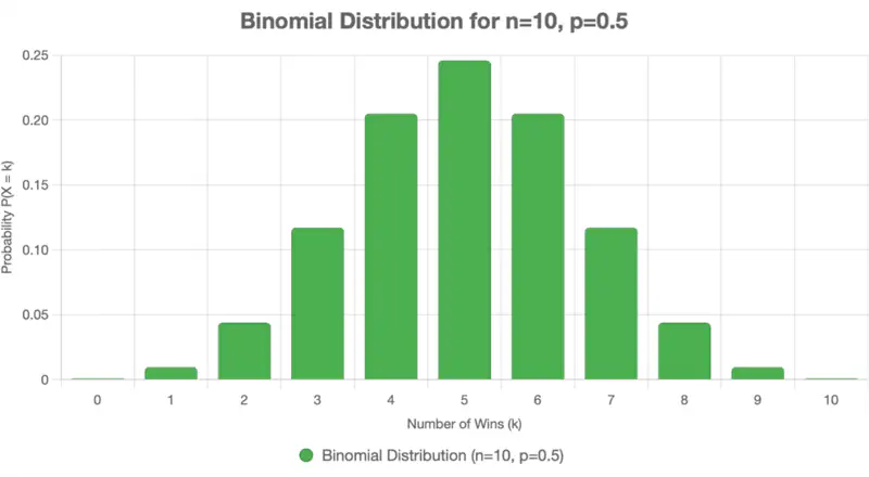
Total number of outcomes in 3 coin tosses = 2^3 = 8
Desired outcomes i.e 2 heads in 3 coin tosses = \(\{HHT, HTH, THH\}\) = 3
Probability of getting exactly 2 heads in 3 coin tosses = \(\frac{3}{8}\) = 0.375
Now lets solve the question using the binomial distribution formula.
Number of successes, k = 1
Number of trials, n = 10
Probability of success, p = 1/3
Probability of winning lottery, P(k=1) =
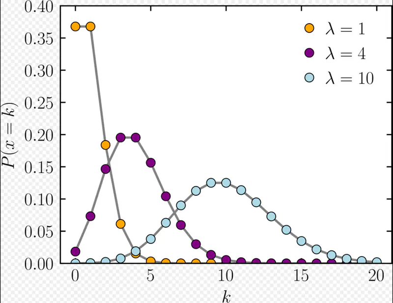
It expresses the probability of an event happening a certain number of times ‘k’ within a fixed interval of time.
Given that:
- Events occur with a known constant average rate.
- Occurrence of an event is independent of the time since the last event.
Parameters:
\(\lambda\): Expected number of events per interval
\(k\) = Number of events in the same interval
Mean = \(\lambda\)
Variance = \(\lambda\)
PMF = Probability of occurrence of ‘k’ events in the same interval
Note: Useful to count data where total population size is large but the probability of an individual event is small.
- Model the number of customers arrival at a service center per hour.
- Number of website clicks in a given time period.
Expected (average) number of emails per hour, \(\lambda\) = 5
Probability of receiving exactly k=3 emails in the next hour =
End of Section
1.6 - Probability Density Function
This is a function used for continuous random variables to describe the likelihood of the variable taking on a value
within a specific range or interval.
Since, at any given point the probability of a continuous random variable is zero,
we find the probability within a given range.
Note: Called ‘density’ because probability is spread continuously over a range of values
rather than being concentrated at a single point as in PMF.
e.g: Uniform, Gaussian, Exponential, etc.
Note: PDF is a continuous function \(f(x)\).
It is also the derivative of Cumulative Distribution Function (CDF) \(F_X(x)\)
\(PDF = f(x) = F'(X) = \frac{dF_X(x)}{dx} \)
- Non-Negative: Function must be non-negative everywhere i.e \(f(x) \ge 0 \forall x\).
- Sum = 1: Total area under curve must be equal to 1.
\( \int_{-\infty}^{\infty} f(x) \,dx = 1\) - Probability of a continuous random variable in the range [a,b] is given by -
\( P(a \le x \le b) = \int_{a}^{b} f(x) \,dx\)
Consider a line segment/interval from \(\Omega = [0,2] \)
Random variable \(X(\omega) = \omega\)
i.e \(X(1) = 1 ~and~ X(1.1) = 1.1 \)
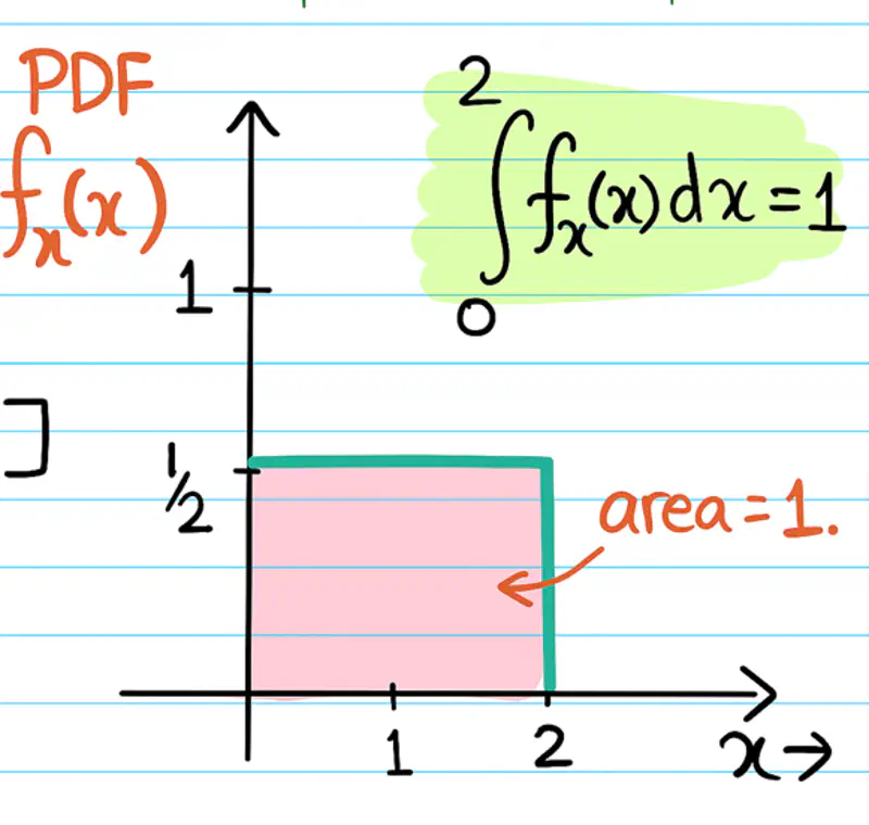
Note: If we know the PDF of a continuous random variable, then we can find the probability of any given region/interval by calculating the area under the curve.
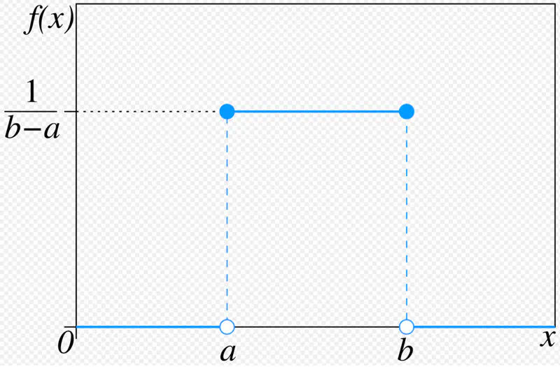
All the outcomes within the given range are equally likely to occur.
Also known as ‘fair’ distribution.
Note: This is a natural starting point to understand randomness in general.
Mean = Median = \( \frac{a+b}{2} ~if~ x \in [a,b] \)
Variance = \( \frac{(b-a)^2}{12} \)
Standard uniform distribution: \( X \sim U(0,1) \)
PDF in terms of mean(\(\mu\)) and standard deviation(\(\sigma\)) -
Random number generator that generates a random number between 0 and 1.
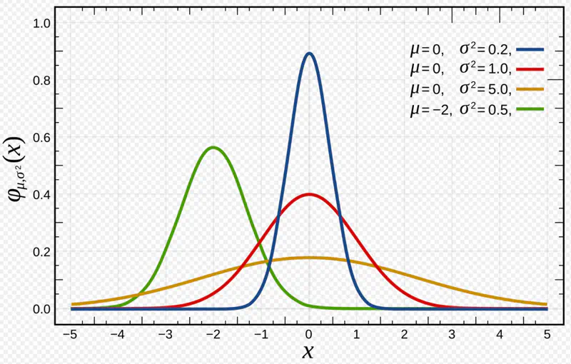
It is a continuous probability distribution characterized by a symmetrical, bell-shaped curve with
most data clustered around the central average, with frequency of values decreasing as they move away from the center.
- Most outcomes are average; extremely low or extremely high values are rare.
- Characterised by mean and standard deviation/variance.
- Peak at mean = median, symmetric around mean.
Note: Most important and widely used distribution.
\[ X \sim N(\mu, \sigma^2) \] $$ \begin{aligned} PDF = f(x) = \dfrac{1}{\sqrt{2\pi}\sigma}e^{-\dfrac{(x-\mu)^2}{2\sigma^2}} \\ \end{aligned} $$
Mean = \(\mu\)
Variance = \(\sigma^2\)
Standard normal distribution:
\[ Z \sim N(0,1) ~i.e~ \mu = 0, \sigma^2 = 1 \]
Any normal distribution can be standardized using Z-score transformation:
- Human height, IQ scores, blood-pressure etc.
- Measurement of errors in scientific experiments.
- 68.27% of the data lie within 1 standard deviation of the mean i.e \(\mu \pm \sigma\)
- 95.45% of the data lie within 2 standard deviations of the mean i.e \(\mu \pm 2\sigma\)
- 99.73% of the data lie within 3 standard deviations of the mean i.e \(\mu \pm 3\sigma\)
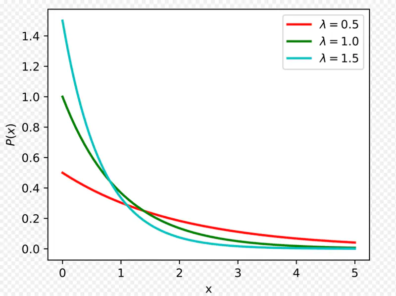
It is used to model the amount of time until a specific event occurs.
Given that:
- Events occur with a known constant average rate.
- Occurrence of an event is independent of the time since the last event.
Parameters:
Rate parameter: \(\lambda\): Average number of events per unit time
Scale parameter: \(\mu ~or~ \beta \): Mean time between events
Mean = \(\frac{1}{\lambda}\)
Variance = \(\frac{1}{\lambda^2}\)
\[ \lambda = \dfrac{1}{\beta} = \dfrac{1}{\mu}\]
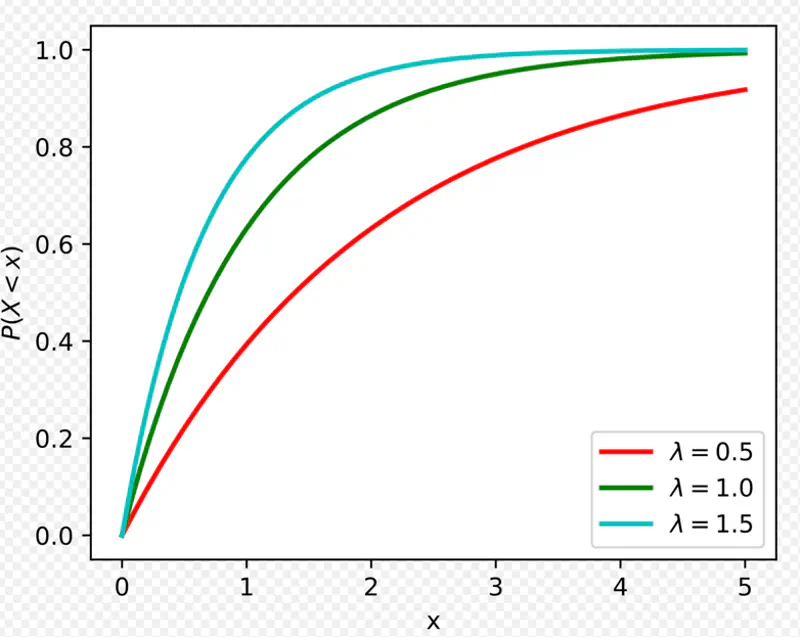
Mean time to serve 1 customer = \(\mu\) = 4 minutes
So, \(\lambda\) = average number of customers served per unit time = \(1/\mu\) = 1/4 = 0.25 minutes
Probability to serve a customer in less than 3 minutes can be found using CDF -
So, probability of a customer being served in less than 3 minutes is 53%(approx).
In this case x = 2 minutes, and \(\lambda\) = 0.25 so,
So, probability of a customer being served in greater than 2 minutes is 60%(approx).
Probability of waiting for an additional period of time for an event to occur is independent of
how long you have already waited.
e.g: Lifetime of electronic items follow exponential distribution.
- Probability of a computer part failing in the next 1 hour is the same regardless of whether
it has been working for 1 day or 1 year or 5 years.
Note: Memoryless property makes exponential distribution particularly useful for -
- Modeling systems that do not experience ‘wear and tear’; where failure is due to a constant random rate rather than degradation over time.
- Also, useful for ‘reliability analysis’ of electronic systems where a ‘random failure’ model is more appropriate than
a ‘wear out’ model.
Task: We want to find the probability of the electronic item lasting for \(x > t+s \) days,
given that it has already lasted for \(x>t\) days.
This is a ‘conditional probability’.
Since,
We want to find: \( P(X > t+s \mid X > t) = ~? \)
Hence, probability that the electronic item will survive for an additional time ’s’ days
is independent of the time ’t’ days it has already survived.
Poisson distribution models the number of events occurring in a fixed interval of time,
given a constant average rate \(\lambda \).
Exponential distribution models the time interval between those successive events.
- 2 faces of the same coin.
- \(\lambda_{poisson}\) is identical to rate parameter \(\lambda_{exponential}\).
Note: If the number of events in a given interval follow a Poisson distribution, then the waiting time between those events will necessarily follow an Exponential distribution.
Lets see the proof for the above statement.
Poisson Case:
The probability of observing exactly ‘k’ events in a time interval of length ’t’
with an average rate of \( \lambda \) events per unit time is given by -
The event that waiting time until next event > t, is same as observing ‘0’ events in that interval.
=> We can use the PMF of Poisson distribution with k=0.
Exponential Case:
Now, lets consider exponential distribution that models the waiting time ‘T’ until next event.
The event that waiting time ‘T’ > t, is same as observing ‘0’ events in that interval.
Observation:
Exponential distribution is a direct consequence of Poisson distribution probability of ‘0’ events.
Using Poisson:
Average failure rate, \(\lambda\) = 1/20 = 0.05
Time interval, t = 10 hours
Number of events, k = 0
Average number of events in interval, (\(\lambda t\)) = (1/20) * 10 = 0.5
Probability of having NO failures in the next 10 hours = ?
Using Exponential:
What is the probability that wait time until next failure > 10 hours?
Waiting time, T > t = 10 hours.
Average number of failures per hour, \(\lambda\) = 1/20 per hour
Therefore, we have seen that this problem can be solved using both Poisson and Exponential distribution.
End of Section
1.7 - Expectation
Long run average of the outcomes of a random experiment.
When we talk about ‘Expectation’ we mean - on an average.
- Value we expect to get when we repeated an experiment multiple times and took an average of the results.
- Measures the central tendency of a data distribution.
- Similar to ‘Center of Mass’ in Physics.
Note: If the probability of each outcome is different, then we take a weighted average.
Discrete Case:
\(E[X] = \sum_{i=1}^{n} x_i.P(X = x_i) \)
Continuous Case:
\(E[X] = \int_{-\infty}^{\infty} x.f(x) dx \)
if its a tail, then you lose Rs. 50. What is the expected value of the amount that you will win per toss?
Possible outcomes are: \(x_1 = 100 ,~ x_2 = -50 \)
Probability of each outcome is \(P(X = 100) = 0.5,~ P(X = -50) = 0.5 \)
Therefore, the expected value of the amount that you will win per toss is Rs. 25 in the long run.
It is the average of the squared differences from the mean.
- Measures the spread or variability in the data distribution.
- If the variance is low, then the data is clustered around the mean i.e less variability;
and if the variance is high, then the data is widely spread out i.e high variability.
Variance in terms of expected value, where \(E[X] = \mu\), is given by:
\[ \begin{aligned} Var[X] &= E[(X - E[X])^2] \\ &= E[X^2 + E[X]^2 - 2XE[X]] \\ &= E[X^2] + E[X]^2 - 2E[X]E[X] \\ &= E[X^2] + E[X]^2 - 2E[X]^2 \\ Var[X] &= E[X^2] - E[X]^2 \\ \end{aligned} \]Note: This is the computational formula for variance, as it is easier to calculate than the
average of square distances from mean.
PDF of continuous uniform random variable =
$$ \begin{aligned} f_X(x) &= \begin{cases} \dfrac{1}{b-a}, & x \in [a,b] \\ 0, & \text{otherwise.} \end{cases} \\ \end{aligned} $$\[ \begin{aligned} \text{Expected value = mean } = \\[0.5em] E[X] = \dfrac{b+a}{2} \\[0.5em] Var[X] = E[X^2] - E[X]^2 \end{aligned} \]We know \(E[X]\) already, now we will calculate \(E[X^2]\):
\[ \begin{aligned} E[X] &= \int_{-\infty}^{\infty} x.f(x) dx \\ E[X^2] &= \int_{-\infty}^{\infty} x^2.f(x) dx \\ &= \int_{-\infty}^{a} x^2f(x) dx + \int_{a}^{b} x^2f(x) dx + \int_{b}^{\infty} x^2f(x) dx\\ &= 0 + \int_{a}^{b} x^2f(x) dx + 0 \\ &= \int_{a}^{b} x^2f(x) dx \\ &= \dfrac{1}{b-a} \int_{a}^{b} x^2 dx \\ &= \dfrac{1}{b-a} * \{\frac{x^3}{3}\}_{a}^{b} \\ &= \dfrac{1}{b-a} * \{\frac{b^3 - a^3}{3}\} \\ &= \dfrac{1}{b-a} * \{\frac{(b-a)(b^2+ab+a^2)}{3}\} \\ E[X^2] &= \dfrac{b^2+ab+a^2}{3} \end{aligned} \]Now, we know both \(E[X]\) and \(E[X^2]\), so we can calculate \(Var[X]\):
\[ \begin{aligned} Var[X] &= E[X^2] - E[X]^2 \\ &= \dfrac{b^2+ab+a^2}{3} - \dfrac{(b+a)^2}{4} \\ &= \dfrac{b^2+ab+a^2}{3} - \dfrac{b^2+2ab+a^2}{4} \\ &= \dfrac{4b^2+4ab+4a^2-3b^2-6ab-3a^2}{12} \\ &= \dfrac{b^2-2ab+a^2}{12} \\ Var[X]&= \dfrac{(b-a)^2}{12} \end{aligned} \]It is the measure of how 2 variables X & Y vary together.
It gives the direction of the relationship between the variables.
Note: For both direction as well as magnitude, we use Correlation.
Let’s use expectation to compute the co-variance of two random variables X & Y:
Note:
- In a multivariate setting, relationship between all the pairs of random variables are summarized in
a square symmetrix matrix called ‘Co-Variance Matrix’ \(\Sigma\).
- Covariance of a random variable with self gives the variance, hence the diagonals of covariance matrix are variances.
End of Section
1.8 - Moment Generating Function
They are statistical measures that describe the characteristics of a probability distribution,
such as its central tendency, spread/variability, and asymmetry.
Note: We will discuss ‘raw’ and ‘central’ moments.
Important moments:
- Mean : Central tendency
- Variance : Spread/variability
- Skewness : Asymmetry
- Kurtosis : Tailedness
It is a function that simplifies computation of moments, such as, the mean, variance, skewness, and kurtosis,
by providing a compact way to derive any moment of a random variable through differentiation.
- Provides an alternative to PDFs and CDFs of random variables.
- A powerful property of the MGF is that its \(n^{th}\) derivative, when evaluated at \((t=0)\) = the \(n^{th}\) moment of the random variable.
Not all probability distributions have MGFs; sometimes, integrals may not converge and moment may not exist.
Since, \(MGF = M_X(t) = E[e^{tX}] \), we can write the MGF as:
Say, \( E[X^n] = m_n \), where \(m_n\) is the \(n^{th}\) moment of the random variable, then:
\[ M_X(t) = 1 + \frac{t}{1!}m_1 + \frac{t^2}{2!}m_2 + \frac{t^3}{3!}m_3 + \cdots + \frac{t^n}{n!}m_n + \cdots \\ \]Important: Differentiating \(M_X(t)\) with respect to \(t\), \(i\) times, and setting \((t =0)\) gives us the \(i^{th}\) moment of the random variable.
\[ \frac{dM_X(t) }{dt} = M'_X(t) = 0 + m_1 + \frac{2t}{2!}m_2 + \frac{3t^2}{3!}m_3 + \cdots + \frac{nt^n-1}{n!}m_n + \cdots \\ \]Set \(t=0\), to get the first moment:
\[ \frac{dM_X(t) }{dt} = M'_X(t) = m_1 \]Similarly, second moment = \(M''_X(t) = m_2 = E[X^2]\)
And, \(n^{th}\) derivative = \(M^{(n)}_X(t) = m_n = E[X^n]\)
e.g: \( Var[X] = M''_X(0) - (M'_X(0))^2 \)
Note: If we know the MGF of a random variable, then we do NOT need to do integration or summation to find the moments.
Continuous:
Discrete:
\[ M_X(t) = E[e^{tX}] = \sum_{i=1}^{\infty} e^{tx} P(X=x) \]End of Section
1.9 - Joint & Marginal
It describes the probability of 2 or more random variables occurring simultaneously.
- The random variables can be from different distributions, such as, discrete and continuous.
Joint CDF:
Discrete Case:
Continuous Case:
Joint PMF:
Key Properties:
- \(P(X = x, Y = y) \ge 0 ~ \forall (x,y) \)
- \( \sum_{i} \sum_{j} P(X = x_i, Y = y_j) = 1 \)
Joint PDF:
Key Properties:
- \(f_{X,Y}(x,y) \ge 0 ~ \forall (x,y) \)
- \( \int_{-\infty}^{\infty} \int_{-\infty}^{\infty} f_{X,Y}(x,y) dy dx = 1 \)
- If we consider 2 random variables, say, height(X) and weight(Y), then the joint distribution will tell us the probability of finding a person having a particular height and weight.
A ball is picked at random from each bag, such that both draws are independent of each other.
Let’s use this example to understand joint probability.
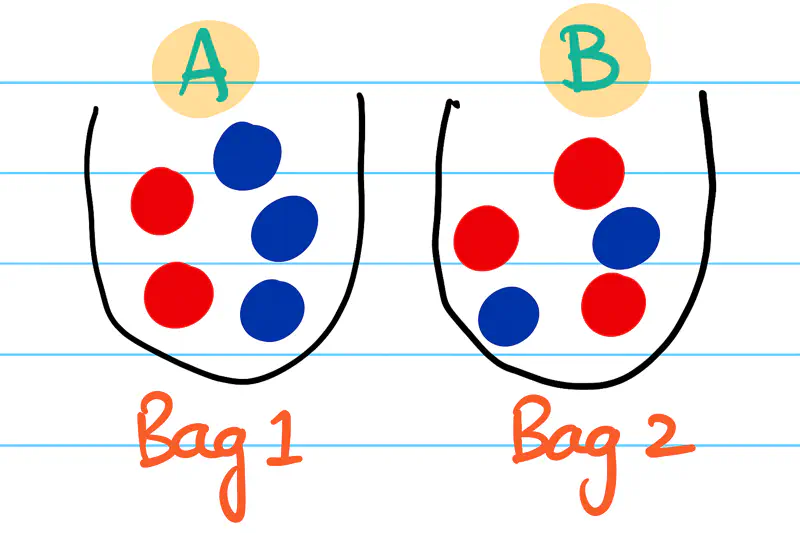
Let A & B be discrete random variables associated with the outcome of the ball drawn from first and second bags
respectively.
| A = Red | A = Blue | |
|---|---|---|
| B = Red | 2/5*3/5 = 6/25 | 3/5*3/5 = 9/25 |
| B = Blue | 2/5*2/5 = 4/25 | 3/5*2/5 = 6/25 |
Since, the draws are independent, joint probability = P(A) * P(B)
Each of the 4 cells in above table shows the probability of combination of results from 2 draws or joint probability.
It describes the probability distribution of an individual random variable in a joint distribution,
without considering the outcomes of other random variables.
- If we have the joint distribution, then we can get the marginal distribution of each random variable from it.
- Marginal probability equals summing the joint probability across other random variables.
Marginal CDF:
We know that Joint CDF =
Marginal CDF =
\[ F_X(a, \infty) = P(X \le a, Y < \infty) = P(X \le a) \]Discrete Case:
Continuous Case:
Law of Total Probability
We know that Joint Probability Distribution =
The events \((Y=y)\) partition the sample space, such that:
- \( (Y=y_1) \cap (Y=y_2) \cap ... \cap (Y=y_n) = \Phi \)
- \( (Y=y_1) \cup (Y=y_2) \cup ... \cup (Y=y_n) = \Omega \)
From Law of Total Probability, we get:
Marginal PMF:
Marginal PDF:
X: Roll a die ; \( \Omega = \{1,2,3,4,5,6\} \)
Y: Toss a coin ; \( \Omega = \{H,T\} \)
Joint PMF = \( P_{X,Y}(x,y) = P(X=x, Y=y) = 1/6*1/2 = 1/12\)
Marginal PMF of X = \( P_X(x) =\sum_{y \in \mathbb{\{H,T\}}} P_{X,Y}(x,y) = = 1/12+1/12 = 1/6\)
=> Marginally, X is uniform over 1-6 i.e a fair die.
Marginal PMF of Y = \( P_Y(y) = \sum_{1}^6 P_{X,Y}(x,y) = 6*(1/12) = 1/2 \)
=> Marginally, Y is uniform over H,T i.e a fair coin.
\( X \sim U(0,1) \)
\( Y \sim U(0,1) \)
Marginal PDF = \(f_X(x) = \int_{-\infty}^{\infty} f_{X,Y}(x,y) dy \)
Joint PDF =
Marginal PDF =
\[ \begin{aligned} f_X(x) &= \int_{0}^{1} f_{X,Y}(x,y) dy \\ &= \int_{0}^{1} 1 dy \\ &= 1 \\ f_X(x) &= \begin{cases} 1 & \text{if } x \in [0,1] \\ 0 & \text{otherwise } \end{cases} \end{aligned} \]There are 2 bags; bag_1 has 2 red balls & 3 blue balls, bag_2 has 3 red balls & 2 blue balls.
A ball is picked at random from each bag, such that both draws are independent of each other.
Let’s use this example to understand marginal probability.
Let A & B be discrete random variables associated with the outcome of the ball drawn from first and second bags
respectively.
| A = Red | A = Blue | P(B) (Marginal) | |
|---|---|---|---|
| B = Red | 2/5*3/5 = 6/25 | 3/5*3/5 = 9/25 | 6/25 + 9/25 = 15/25 = 3/5 |
| B = Blue | 2/5*2/5 = 4/25 | 3/5*2/5 = 6/25 | 4/25 + 6/25 = 10/25 = 2/5 |
| P(A) (Marginal) | 6/25 + 4/25 = 10/25 = 2/5 | 9/25 + 6/25 = 15/25 = 3/5 |
We can see from the table above - P(A=Red) is the sum of joint distribution over all possible values of B i.e Red & Blue.
It measures the probability of an event occurring given that another event has already happened.
- It provides a way to update our belief about the likelihood based on new information.
P(A, B) = Joint Probability of A and B
P(B) = Marginal Probability of B
=> Conditional Probability = Joint Probability / Marginal Probability
Conditional CDF:
Discrete Case:
Continuous Case:
Conditional PMF:
Conditional PDF:
- Generative machine learning models, such as, GANs, learn the conditional distribution of pixels, given the style of input image.
Note: We only have information about the joint and marginal probabilities.
What is the conditional probability of drawing a red ball in the first draw, given that a blue ball is drawn in second draw?
Let A & B be discrete random variables associated with the outcome of the ball drawn from first and second bags
respectively.
A = Red ball in first draw
B = Blue ball in second draw.
| A = Red | A = Blue | P(B) (Marginal) | |
|---|---|---|---|
| B = Red | 6/25 | 9/25 | 3/5 |
| B = Blue | 4/25 | 6/25 | 2/5 |
| P(A) (Marginal) | 2/5 | 3/5 |
Therefore, probability of drawing a red ball in the first draw, given that a blue ball is drawn in second draw = 2/5.
This gives us the conditional expectation of a random variable X, given another random variable Y=y.
Discrete Case:
Continuous Case:
- Conditional expectation of of a person’s weight, given his/her height = 165 cm, will give us the average weight of all people with height = 165 cm.
Applications:
- Linear regression algorithm is conditional expectation of target variable ‘Y’, given input feature variable ‘X’.
- Expectation Maximisation(EM) algorithm is built on conditional expectation.
This gives us the variance of a random variable calculated after taking into account the value(s) of another related variable.
For example:
- Variance of car’s mileage for city driving might be small, but the variance will be large for mix of city and highway driving.
Note: Models that take into account the change in variance or heteroscedasticity tend to be more accurate.
End of Section
1.10 - Independent & Identically Distributed
Let’s revisit and understand the independence of random variables first.
It means that the knowing the outcome of one random variable does not impact the probability of the other random variable.
Two random variables X & Y are independent if:
- We know that if 2 random variables X,Y are independent, then their covariance is zero,
since there is no linear relationship between them.
- But the converse may NOT be true, i.e, if the covariance is zero, then we can say for sure that the random variables
are independent.
Let’s go through few examples to understand the independence of random variables.
For example:
- Toss a coin + Roll a die.
\[ X = \begin{cases} 1 & \text{if Heads} \\ \\ 0 & \text{if Tails} \end{cases} \\ \text{} \\ Y = \{1,2,3,4,5,6\} \\ \text{} \\ \text{ Joint probability is all possible combinations of X and Y i.e 2x6 = 12 } \\[10pt] \text{ Sample space: } \Omega = \{ (H,1), (H,2), (H,3), (H,4), (H,5), (H,6), \\ (T,1), (T,2), (T,3), (T,4), (T,5), (T,6) \} \]
Here, clearly, X and Y are independent.
- Toss a coin twice.
\(X\) = Number of heads = \(\{0,1,2\}\)
\(Y\) = Number of tails = \(\{0,1,2\}\)
X, Y are NOT independent, but mutually exclusive, because if we know about one, then we automatically know about the other.
- \(X\) is a continuous uniform random variable \( X \sim U(-1,1) \).
\(Y = 2X\).
Let’s check for independence of \(X\) and \(Y\) i.e \(E[XY] = E[X]E[Y]\) or not?
Now, lets calculate the value of \(E[XY]\):
From (1) and (2), we can say that:
\[ E[XY] ⍯ E[X]E[Y] \\ \]Hence, \(X\) and \(Y\) are NOT independent.
Read more about Integration
Similarly, random variables X & Y are said to be identically distributed if they belong to the same probability distribution.
I.I.D assumption for samples(data points) in a dataset means that the samples are:
- Independent, i.e, each sample is independent of the other.
- Identically distributed, i.e, each sample is drawn from the same probability distribution.
- We take the heights of a random sample of people to estimate the average height of the population of a city.
- Here ‘independent’ assumption means that the height of each person in the sample is independent of the other person.
Usually, heights of members of the same family may be highly correlated.
However, for practical purposes, we can assume that all the heights are independent of one another. - And, for ‘identically distributed’ - we can assume that all the heights are from the same Gaussian distribution with some mean and variance.
- Here ‘independent’ assumption means that the height of each person in the sample is independent of the other person.
End of Section
1.11 - Convergence
A sequence of random variables \(X_1, X_1, \dots, X_n\) is said to converge in probability
to a known random variable \(X\),
if for every number \(\epsilon >0 \), the following is true:
where,
\(X_n\): is the estimator or sample based random variable.
\(X\): is the known or limiting or target random variable.
\(\epsilon\): is the tolerance level or margin of error.
- Toss a fair coin:
Estimator:
\[ X_n = \begin{cases} \frac{n}{n+1} & \text{, if Head } \\ \\ \frac{1}{n} & \text{, if Tail} \\ \end{cases} \]
Known random variable (Bernoulli):
\[ X = \begin{cases} 1 & \text{, if Head } \\ \\ 0 & \text{, if Tail} \\ \end{cases} \]
Say, tolerance level \(\epsilon = 0.1\).
Then,
If n=5;
So, if n=5, then \(|X_n - X| > (\epsilon = 0.1)\).
\( \implies P(|X_n - X| \ge (\epsilon=0.1)) = 1\).
if n=20;
So, if n=20, then \(|X_n - X| < (\epsilon=0.1)\).
\(\implies P(|X_n - X| \ge (\epsilon=0.1)) = 0\).
\( \implies P(|X_n - X| \ge (\epsilon=0.1)) = 0 ~\forall ~n \ge 10\)
Therefore,
Similarly, we can prove that if \(\epsilon = 0.01\), then the probability will be equal to 0 for \( n\ge 100 \).
Note: Task is to check whether the sequence of randome variables \(X_1, X_2, \dots, X_n\) converges in probability to a known random variable \(X\) as \(n\rightarrow\infty\).
So, we can conclude that, if \(n > \frac{1}{\epsilon}\), then:
A sequence of random variables \(X_1, X_2, \dots, X_n\) is said to almost surely converge to a known random variable \(X\),
for \(n \ge 1\), if the following is true:
where,
\(X_n\): is the estimator or sample based random variable.
\(X\): is the known or limiting or target random variable.
If, \(X_n \xrightarrow{Almost ~ Sure} X \), \( \implies X_n \xrightarrow{Probability} X \)
But, converse is NOT true.
*Note: Almost Sure convergence is hardest to satisfy amongst all convergence, such as, convergence in probability,
convergence in distribution, etc.
Read more about Limits
- \(X\) is random variable such that \(X = \frac{1}{2} \), a constant, i.e \(X_1 = X_2 = \dots = X_n = \frac{1}{2}\).
\(Y_1, Y_2,\dots ,Y_n \) are another sequence of random variables, such that :
\[ Y_1 = X_1 \\[10pt] Y_2 = \frac{X_1 + X_2}{2} \\[10pt] Y_3 = \frac{X_1 + X_2 + X_3}{3} \\[10pt] \dots \\ Y_n = \frac{1}{n} \sum_{i=1}^{n} X_i \xrightarrow{Almost ~ Sure} \frac{1}{2} \]
End of Section
1.12 - Law of Large Numbers
This law states that given a sequence of independent and identically distributed (IID) samples \(X_1, X_1, \dots, X_n\) from a random variable with finite mean, the sample mean (\(\bar{X_n}\)) converges in probability to the expected value \(E[X]\) or population mean (\( \mu \)).
\[ \lim_{n\rightarrow\infty} P(|\bar{X_n} - E[X]| \ge \epsilon) = 0, \forall ~ \epsilon >0 \\[10pt] \\[10pt] \frac{1}{n} \sum_{i=1}^{n} X_i \xrightarrow{Probability} E[X], \text{ as } n \rightarrow \infty \]Note: Does NOT guarantee that sample mean will be close to population mean,
but instead says that - the probability of sample mean being far away from the population mean is low.
Read more about Limits
- Toss a coin large number of times \('n'\), as \(n \rightarrow \infty\), the proportion of heads will probably be very
close to \(0.5\).
However, it does NOT rule out the possibility of a rare sequence, e.g., getting 10 consecutive heads.
But, the probability of such a rare event is extremely low.
This law states that given a sequence of independent and identically distributed (IID) samples \(X_1, X_1, \dots, X_n\) from a random variable with finite mean, the sample mean (\(\bar{X_n}\)) converges almost surely to the expected value \(E[X]\) or population mean (\( \mu \)).
\[ P(\lim_{n\rightarrow\infty} \bar{X_n} = E[X]) = 1, \text{ as } n \rightarrow \infty \\[10pt] \frac{1}{n} \sum_{i=1}^{n} X_i \xrightarrow{Almost ~ Sure} E[X], \text{ as } n \rightarrow \infty \]Note:
- It guarantees that the sequence of sample averages itself converges to population mean, with exception of set of outcomes that has probability = 0.
- Almost certain guarantee; Much stronger statement than Weak Law of Large Numbers.
- Toss a coin large number of times \('n'\), as \(n \rightarrow \infty\), the proportion of heads will converge
to \(0.5\), with probability = 1.
This means that a sequence where the proportion of heads never settles down to 0.5, is a probability = 0 event.
- Almost sure convergence ensures ML model’s reliability by guaranteeing that the average error on a large dataset will
converge to the true error.
Thus, providing confidence that model will perform consistently and accurately on unseen data.
End of Section
1.13 - Markov's Inequality
It gives an upper bound for the probability that a non-negative random variable will NOT exceed, based on its expected value.
Note: It gives a very loose upper bound.
Read more about Expectation
What is the probability that the restaurant will serve more than 200 customers in the next hour?
Hence, a 25% chance of serving more than 200 customers.
What is the probability that a randomly selected student gets a score of 90 marks or more?
Hence, there is a 78% chance that a randomly selected student gets a score of 90 marks or more.
It states that the probability of a random variable deviating from its mean is small if its variance is small.
- It is a more powerful version of Markov’s Inequality.
- It uses variance of the distribution in addition to the expected value or mean.
- Also, it does NOT assume the random variable to be non-negative.
- It uses more information about the data i.e mean and variance.
Note: It gives a tighter upper bound than Markov’s Inequality.
What is the probability that a randomly selected student gets a score of 90 marks or more?
Given the standard deviation of the test score is 10 marks.
Given, the standard deviation of the test score \(\sigma\) = 10 marks.
=> Variance = \(\sigma^2\) = 100
Hence, Chebyshev’s Inequality gives a far tighter upper bound of 25% than Markov’s Inequality of 78%(approx).
It is an upper bound on the probability that a random variable deviates from its expected value.
It’s an exponentially decreasing bound on the “tail” of a random variable’s distribution,
which can be calculated using its moment generating function.
- It is used for sum or average of independent random variables (not necessarily identically distributed).
- It provides exponentially tighter bounds, better than Chebyshev’s Inequality’s quadratic decay.
- It uses all moments to capture the full shape of the distribution, using the moment generating function(MGF).
Proof:
For the sum of ’n’ independent random variables,
Note: Used to compute how far the sum of independent random variables deviate from their expected value.
Read more about Moment Generating Function
End of Section
1.14 - Cross Entropy & KL Divergence
It is a measure of the amount of information gained when a specific, individual event occurs, and is defined based on
the probability of that event.
It is defined as the negative logarithm of the probability of the event.
- It is also called ‘Surprisal’.
Note: Logarithm(for base > 1) is a monotonically increasing function, so as x increases, log(x) also increases.
- So, if probability P(x) increases, then surprise factor S(x) decreases.
- Common events have a high probability of occurrence, hence a low surprise factor.
- Rare events have a low probability of occurrence, hence a high surprise factor.
Units:
- The unit of surprise factor with log base 2 is bits.
- with base ’e’ or natural log its nats (natural units of information).
It conveys how much ‘information’ we expect to gain from a random event.
- Entropy is the average or expected value of surprise factor of a random variable.
- More uniform the distribution ⇒ greater average surprise factor, since all possible outcomes are equally likely.
Case 1:
Toss a fair coin; \(P(H) = P(T) = 0.5 = 2^{-1}\)
Surprise factor (Heads or Tails) = \(-log(P(x)) = -log_2(0.5) = -log_2(2^{-1}) = 1~bit\)
Entropy = \( \sum_{x \in X} P(x)log(-P(x)) = 0.5*1 + 0.5*1 = 1 ~bit \)Case 2:
Toss a biased coin; \(P(H) = 0.9 P(T) = 0.1 \)
Surprise factor (Heads) = \(-log(P(x)) = -log_2(0.9) \approx 0.15 ~bits \)
Surprise factor (Tails) = \(-log(P(x)) = -log_2(0.1) \approx 3.32 ~bits\)
Entropy = \( \sum_{x \in X} P(x)log(-P(x)) = 0.9*0.15 + 0.1*3.32 \approx 0.47 ~bits\)
Therefore, a biased coin is less surprising on an average than a fair coin, hence lower entropy.
It is a measure of the average ‘information gain’ or ‘surprise’ when using an imperfect model \(Q\) to encode events
from a true model \(P\).
- It measures how surprised we are on an average, if the true distribution is \(P\), but we predict using another distribution
\(Q\).
A model is trained to classify images as ‘cat’ or ‘dog’. Say, for an input image the true label is ‘cat’,
so the true distribution:
\(P = [1.0 ~(cat), 0.0 ~(dog)]\).
Let’s calculate the cross-entropy for the outputs of 2 models A & B.
Model A:
\(Q_A = [0.8 ~(cat), 0.2 ~(dog)]\)
Cross Entropy = \(H(P, Q_A) = -\sum_{i=1}^n P(x_i)log(Q_A(x_i)) \)
\(= -[1*log_2(0.8) + 0*log_2(0.2)] \approx 0.32 ~bits\)
Note: This is very low cross-entropy, since the predicted value is very close to actual, i.e low surprise.Model B:
\(Q_B = [0.2 ~(cat), 0.8 ~(dog)]\)
Cross Entropy = \(H(P, Q_B) = -\sum_{i=1}^n P(x_i)log(Q_B(x_i)) \)
\(= -[1*log_2(0.2) + 0*log_2(0.8)] \approx 2.32 ~bits\)
Note: Here the cross-entropy is very high, since the predicted value is quite far from the actual truth, i.e high surprise.
It measures the information lost when one probability distribution \(Q\) is used to approximate another distribution \(P\).
It quantifies the ‘extra cost’ in bits needed to encode data using the approximate distribution \(Q\) instead of
the true distribution \(P\).
KL Divergence = Cross Entropy(P,Q) - Entropy(P)
\[ \begin{aligned} D_{KL}(P \parallel Q) &= H(P, Q) - H(P) \\ &= -\sum_{i=1}^n P(x_i)log(Q(x_i)) - [-\sum_{i=1}^n P(x_i)log(P(x_i))] \\[10pt] &= \sum_{i=1}^n P(x_i)[log(P(x_i)) - log(Q(x_i)) ] \\[10pt] D_{KL}(P \parallel Q) &= \sum_{i=1}^n P(x_i)log(\frac{P(x_i)}{Q(x_i)}) \\[10pt] \text{ For continuous case: } \\ D_{KL}(P \parallel Q) &= \int_{-\infty}^{\infty} p(x)log(\frac{p(x)}{q(x)})dx \end{aligned} \]Note:
- If \(P = Q\) ,i.e, P and Q are the same distributions, then KL Divergence = 0.
- KL divergence is NOT symmetrical ,i.e, \(D_{KL}(P \parallel Q) ⍯ (D_{KL}(Q \parallel P)\).
Using the same cat, dog classification problem example as mentioned above.
A model is trained to classify images as ‘cat’ or ‘dog’. Say, for an input image the true label is ‘cat’,
so the true distribution:
\(P = [1.0 ~(cat), 0.0 ~(dog)]\).
Let’s calculate the KL divergence for the outputs of the 2 models A & B.
Let’s calculate entropy first, and we can reuse the cross-entropy values calculated above already.
Entropy: \(H(P) = -\sum_{x \in X} P(x)log(P(x)) = -[1*log_2(1) + 0*log_2(0)] = 0 ~bits\)
Note: \(0*log_2(0) = 0\), is an approximation hack, since \(log(0)\) is undefined.
Model A:
\( D_{KL}(P \parallel Q) = H(P, Q) - H(P) = 0.32 - 0 = 0.32 ~bits \)
Model A incurs an additional 0.32 bits of surprise due to its imperfect prediction.Model B:
\( D_{KL}(P \parallel Q) = H(P, Q) - H(P) = 2.32 - 0 = 2.32 ~bits \)
Model B has much more ‘information loss’ or incurs higher ‘penalty’ of 2.32 bits as its prediction was from from the truth.
It is a smoothed and symmetric version of the Kullback-Leibler (KL) divergence and is calculated by averaging the
KL divergences between each of the two distributions and their combined average distribution.
- Symmetrical and smoothed version of KL divergence.
- Always finite; KL divergence can be infinite if \( P ⍯ 0 ~and~ Q = 0 \).
- Makes JS divergence more stable for ML models where some predicted probabilities may be exactly 0.
Let’s continue the cat and dog image classification example discussed above.
A model is trained to classify images as ‘cat’ or ‘dog’. Say, for an input image the true label is ‘cat’,
so the true distribution:
\(P = [1.0 ~(cat), 0.0 ~(dog)]\).
Step 1: Calculate the average distribution M.
Step 2: Calculate \(D_{KL}(P \parallel M)\).
Step 3: Calculate \(D_{KL}(Q \parallel M)\).
Step 4: Finally, lets put all together to calculate \(D_{JS}(P \parallel Q)\).
Therefore, lower JS divergence value => P and Q are more similar.
End of Section
1.15 - Parametric Model Estimation
It is the process of finding the best-fitting finite set of parameters \(\Theta\) for a model that assumes a
specific probability distribution for the data.
It involves using the dataset to estimate the parameters (like the mean and standard deviation of a normal distribution)
that define the model.
\(P(X \mid \Theta) \) : Probability of seeing data \(X: (X_1, X_2, \dots, X_n) \), given the parameters \(\Theta\) of the
underlying probability distribution from which the data is assumed to be generated.
Goal of estimation:
We observed data, \( D = \{X_1, X_2, \dots, X_n\} \), and we want to infer the the unknow parameters \(\Theta\)
of the underlying probability distribution, assuming that the data is generated I.I.D.
Read more for I.I.D
Note: Most of the time, from experience, we know the underlying probability distribution of data, such as, Bernoulli, Gaussian, etc.
There are 2 philosophical approaches to estimate the parameters of a parametric model:
- Frequentist:
- Parameters \(\Theta\) is fixed, but unknown, only data is random.
- It views probability as the long-run frequency of events in repeated trials; e.g toss a coin ’n’ times.
- It is favoured when the sample size is large.
- For example, Maximum Likelihood Estimation(MLE), Method of Moments, etc.
- Bayesian:
- Parameters \(\Theta\) itself is unknown, so we model it as a random variable with a probability distribution.
- It views probability as a degree of belief that can be updated with new evidence, i.e. data.
Thus, integrating prior knowledge with data to express the uncertainty about the parameters. - It is favoured when the sample size is small, as it uses prior belief about the data distribution too.
- For example, Maximum A Posteriori Estimation(MAP), Minimum Mean Square Error Estimation(MMSE), etc..
It is the most popular frequentist approach to estimate the parameters of a model.
This method helps us find the parameters \(\Theta\) that make the data most probable.
Likelihood Function:
Say, we have data, \(D = X_1, X_2, \dots, X_n\) are I.I.D discrete random variable with PMF = \(P_{\Theta}(.)\)
Then, the likelihood function is the probability of observing the data, \(D = \{X_1, X_2, \dots, X_n\}\),
given the parameters \(\Theta\).
Task:
Find the value of parameter \(\Theta_{ML}\) that maximizes the likelihood function.
In order to find the parameter \(\Theta_{ML}\) that maximises the likelihood function,
we need to take the first derivative of the likelihood function with respect to \(\Theta\) and equate it to zero.
But, taking derivative of a product is challenging, so we will take the logarithm on both sides.
Note: Log is a monotonically increasing function, i.e, as x increases, log(x) increases too.
Let us denote the log-likelihood function as \(\bar{L}\).
\[ \begin{aligned} \mathcal{\bar{L}_{X_1, X_2, \dots ,X_n}}(\Theta) &= log [\prod_{i=1}^{n} P_{\Theta}(X_i)] \\ &= \sum_{i=1}^{n} log P_{\Theta}(X_i) \\ \end{aligned} \]Therefore, Maximum Likelihood Estimation is the parameter \(\Theta_{ML}\) that maximises the log-likelihood function.
\[ \Theta_{ML}(X_1, X_2, \dots, X_n) = \underset{\Theta}{\mathrm{argmax}}\ \bar{L}_{X_1, X_2, \dots ,X_n}(\Theta) \]Given \(X_1, X_2, \dots, X_n\) are I.I.D. Bernoulli random variable with PMF as below:
Estimate the parameter \(\theta\) using Maximum Likelihood Estimation.
Let, \(n_1 = \) number of 1’s in the dataset.
Likelihood Function:
Log-Likelihood Function:
Maximum Likelihood Estimation:
In order to find the parameter \(\theta_{ML}\), we need to take the first derivative of the log-likelihood function
with respect to \(\theta\) and equate it to zero.
Read more about Derivative
Say, e.g., we have 10 observations for the Bernoulli random variable as: 1,0,1,1,0,1,1,0,1,0.
Then, the parameter \(\Theta_{ML} = \frac{6}{10} = 0.6\) i.e proportion of 1’s.
\(x_1, x_2, \dots, x_n\) are the realisations/observations of the random variable.
Estimate the parameters \(\mu\) and \(\sigma\) of the Gaussian distribution using Maximum Likelihood Estimation.
Likelihood Function:
Log-Likelihood Function:
Note: Here, the first term \( -\frac{n}{2} log (2\pi) \) is a constant wrt both \(\mu\) and \(\sigma\), so we can ignore the term.
Maximum Likelihood Estimation:
Instead of finding \(\mu\) and \(\sigma\) that maximises the log-likelihood function,
we can find \(\mu\) and \(\sigma\) that minimises the negative of the log-likelihood function.
Now, lets differentiate the log likelihood function wrt \(\mu\) and \(\sigma\) separately to get \(\mu_{ML}, \sigma_{ML}\).
Lets, calculate \(\mu_{ML}\) first by taking the derivative of the log-likelihood function wrt \(\mu\) and equating it to 0.
Read more about Derivative
Similarly, we can calculate \(\sigma_{ML}\) by taking the derivative of the log-likelihood function wrt \(\sigma\)
and equating it to 0.
Note: In general MLE is biased, i.e does NOT give an unbiased estimate => divides by \(n\) instead of \((n-1)\).
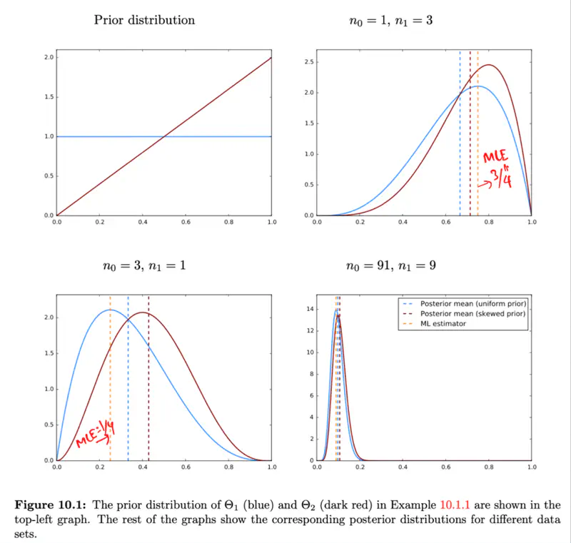
Bayesian statistics model parameters by updating initial beliefs (prior probabilities) with observed data to form
a final belief (posterior probability) using Bayes’ Theorem.
Instead of a single point estimate, it provides a probability distribution over possible parameter values,
which allows to quantify uncertainty and yields more robust models, especially with limited data.
Bayes’ Theorem:
Read more about Bayes’ Theorem
\(P(\Theta)\): Prior: Initial distribution of \(\Theta\) before seeing the data.
\(P(X \mid \Theta)\): Likelihood: Conditional distribution of data \(X\), given the parameter \(\Theta\).
\(P(\Theta \mid X)\): Posterior: Conditional distribution of parameter \(\Theta\), given the data \(X\).
\(P(X)\): Evidence: Probability of seeing the data \(X\).
\(x_1, x_2, \dots, x_n\) are the realisations, \(\Theta \in [0, 1] \).
Estimate the parameter \(\Theta\) using Bayesian statistics.
Let, \(n_1 = \) number of 1’s in the dataset.
Prior: \(P(\Theta)\) : \(\Theta \sim U(0, 1) \), i.e, parameter \(\Theta\) comes from a continuos uniform
distribution in the range [0,1].
\(f_{\Theta}(\theta) = 1, \theta \in [0, 1] \)
Likelihood: \(P_{X \mid \Theta}(x \mid \theta) = \theta^{n_1} (1 - \theta)^{n - n_1} \).
Posterior:
\[ f_{\Theta \mid X} (\theta \mid x) = \frac{f_{\Theta}(\theta) P_{X \mid \Theta}(x \mid \theta)}{f_{X}(x)} \\ \]Note: The most difficult part is to calculate the denominator \(f_{X}(x)\).
So, either we try NOT to compute it all together, or we try to map it to some known functions to make calculations easier.
We know that we can get the marginal probability by integrating the joint probability over another variable.
Also from conditional probability, we know:
\[ \tag{2} f_{X \mid Y}(x \mid y) = \frac{f_{X,Y}(x,y)}{f_{Y}(y)} \\ => f_{X,Y}(x,y) = f_{Y}(y) f_{X \mid Y}(x \mid y) \]From equations 1 and 2, we have:
\[ \tag{3} f_{X}(x) = \int_{Y}f_{Y}(y) f_{X \mid Y}(x \mid y)dy \]Now let’s replace the value of \(f_{X}(x) \) in the posterior from equation 3:
Posterior:
Beta Function:
It is a special mathematical function denoted by B(a, b) or β(a, b) that is defined by the integral formula:
Note: We can see that the denominator of the posterior is of the form of Beta function.
Posterior:
Suppose, in the above example, we are told that the parameter \(\Theta\) is closer to 1 than 0.
How will we incorporate this useful information (apriori knowledge) into our parameter estimation?
Since, we know apriori that \(\Theta\) is closer to 1 than 0, we should take this initial belief into account
to do our parameter estimation.
Prior:
Posterior:
\[ \begin{aligned} f_{\Theta \mid X} (\theta \mid x) &= \frac{f_{\Theta}(\theta) P_{X \mid \Theta}(x \mid \theta)}{f_{X}(x)} \\[10pt] &= \frac{f_{\Theta}(\theta) P_{X \mid \Theta}(x \mid \theta)}{\int_{\Theta}f_{\Theta}(\theta) P_{X \mid \Theta}(x \mid \theta)d\theta} \\[10pt] &= \frac{f_{\Theta}(\theta) P_{X \mid \Theta}(x \mid \theta)}{\int_{0}^1f_{\Theta}(\theta) P_{X \mid \Theta}(x \mid \theta)d\theta} \\[10pt] \text{ We know that: } f_{\Theta}(\theta) = 2\Theta, \theta \in [0, 1] \\ &= \frac{2\Theta * P_{X \mid \Theta}(x \mid \theta)}{\int_{0}^1 2\Theta* P_{X \mid \Theta}(x \mid \theta)d\theta} \\[10pt] & = \frac{2\Theta * \theta^{n_1} (1 - \theta)^{n - n_1}}{\int_{0}^1 2\Theta * \theta^{n_1} (1 - \theta)^{n - n_1}} \\[10pt] => f_{\Theta \mid X} (\theta \mid x) &= \frac{\theta^{n_1+1} (1 - \theta)^{n - n_1}}{β(n_1+2, n-n_1+1)} \end{aligned} \]Note: If we do NOT have enough data, then we should NOT ignore our initial belief.
However, if we have enough data, then the data will override our initial belief and the posterior will be dominated by data.
Note: Bayesian approach gives us a probability distribution of parameter \(\Theta\).
We can use Bayesian Point Estimators, after getting the posterior distribution, to summarize it with a single value for
practical use, such as,
- Maximum A Posteriori (MAP) Estimator
- Minimum Mean Square Error (MMSE) Estimator
It finds the mode(peak) of the posterior distribution.
- MAP has the minimum probability of error, since it picks single most probable value.
Estimate the unknown parameter \(\mu\) using MAP.
Given that :
\(\Theta\) is discrete, with probability 0.5 for both 0 and 1.
=> The Gaussian distribution is equally likely to be centered at 0 or 1.
Variance: \(\sigma^2 = 1\)
Prior:
Likelihood:
Posterior:
We need to find:
\[ \underset{\Theta}{\mathrm{argmax}}\ P_{\Theta \mid X} (\theta \mid x) \]Taking log on both sides:
Let’s calculate the log-likelihood function first -
\[ \begin{aligned} \log f_{X \mid \Theta}(x \mid \theta) &= \log \prod_{i=1}^n \frac{1}{\sqrt{2\pi}} e^{-\frac{(x_i-\theta)^2}{2}} \\ &= log(\frac{1}{\sqrt{2\pi}})^n + \sum_{i=1}^n \log (e^{-\frac{(x_i-\theta)^2}{2}}), \text{ since \(\sigma = 1\)} \\ &= n\log(\frac{1}{\sqrt{2\pi}}) + \sum_{i=1}^n -\frac{(x_i-\theta)^2}{2} \\ => \tag{2} \log f_{X \mid \Theta}(x \mid \theta) &= n\log(\frac{1}{\sqrt{2\pi}}) - \sum_{i=1}^n \frac{(x_i-\theta)^2}{2} \end{aligned} \]Here computing \(f_{X}(x)\) is difficult.
So, instead of differentiating above equation wrt \(\Theta\), and equating to 0,
we will calculate the above expression for \(\theta=0\) and \(\theta=1\) and compare the values.
This way we can get rid of the common value \(f_{X}(x)\) in both expressions that is not dependent on \(\Theta\).
When \(\theta=1\):
Similarly, when \(\theta=0\):
So, we can say that \(\theta = 1\) only if :
the value of the above expression for \(\theta = 1\) > the value of the above expression for \(\theta = 0\)
From equation 3 and 4:
Note: If the prior is uniform then \(\Theta_{MAP} = \Theta_{MLE}\), because uniform prior does NOT give any information about the initial bias, and all possibilities are equally likely.
What if, in the above example, we know that the initial belief is not uniform but biased towards 0?
Prior:
Now, let’s compare the log-posterior for both the cases i.e \(\theta=0\) and \(\theta=1\) as we did earlier.
But, note that this time the probabilities for \(\theta=0\) and \(\theta=1\) are different.
So, we can say that \(\theta = 1\) only if :
the value of the above expression for \(\theta = 1\) > the value of the above expression for \(\theta = 0\)
From equation 3 and 4 above:
Therefore, we can see that \(\Theta_{MAP}\) is extra biased towards 0.
Note: For a non-uniform prior \(\Theta_{MAP}\) estimate will be pulled towards the prior’s mode.
e.g: Patient has a certain disease or not.
But, what if we want to minimize average magnitude of errors, over time, say predicting a stock’s price?
Just getting to know whether the prediction was right or wrong is not sufficient here.
We also want to know that the prediction was wrong by how much, so that we can minimize the loss over time.
Minimizes the expected value of squared error.
Mean of the posterior distribution is the conditional expectation of parameter \(\Theta\), given the data.
- Posterior mean minimizes the the mean squared error.
\(\hat\Theta(X)\): Predicted value.
\(\Theta\): Actual value.
Let’s revisit the above examples that we used for MLE.
Case 1: Uniform Continuous Prior for parameter \(\Theta\) of Bernoulli distribution
Prior:
Posterior:
Let’s calculate the \(\Theta_{MMSE}\):
Similarly, for the second case where the prior is biased towards 1.
Case 2: Prior is biased towards 1 for parameter \(\Theta\) of Bernoulli distribution
Prior:
Posterior:
So, here in this case our \(\Theta_{MMSE}\) is:
- MMSE is the average of the posterior distribution, whereas MAP is the mode/peak.
- If posterior distribution is symmetric and unimodal (only 1 peak), then MAP and MMSE are very close.
- If posterior distribution is skewed and multimodal (many peaks), then MAP and MMSE can differ a lot.
- MMSE considers all the values of the posterior distribution; hence, it is more accurate than MAP, especially for skewed or multimodal distributions.
End of Section
2.1 - Data Distribution
A single number that describes the central, typical, or representative value of a dataset, e.g, mean, median, and mode.
The mean is the average, the median is the middle value in a sorted list, and the mode is the most frequently occurring value.
- A single representative value can be used to compare different groups or distributions.
The artihmetic average of a set of numbers i.e sum all values and divide by the number of values.
\(mean = \frac{1}{n}\sum_{i=1}^{n}x_i\)
- Most common measure of central tendency.
- Represents the ‘balancing point’ of data.
- Sample mean is denoted by \(\bar{x}\), and population mean by \(\mu\).
Pros:
- Uses all datapoints in its calculation, providing a comprehensive measure.
Cons:
- Highly sensitive to outliers i.e exteme values.
- mean\((1,2,3,4,5) = \frac{1+2+3+4+5}{5} = 3 \)
- With outlier: mean\((1,2,3,4,100) = \frac{1+2+3+4+100}{5} = \frac{110}{5} = 22\)
Note: Just a single extreme value of 100 has pushed the mean from 3 to 22.
The middle value of a sorted list of numbers. It divides the dataset into 2 equal halves.
Calculation:
- Arrange the data points in ascending order.
- If the number of data points is even, the median is the average of the two middle values.
- If the number of data points is odd, the median is the middle value i.e \((\frac{n+1}{2})^{th}\) element.
Pros:
- Not impacted by outliers, making it a more robust/reliable measure, especially for skewed distributions.
Cons:
- Does NOT use all the datapoints in its calculation.
- median\((1,2,3,4,5) = 3\)
- median\((1,2,3,4,5,6) = \frac{3+4}{2} = 3.5\)
- With outlier: median\((1,2,3,4,100) = 3\)
Note: No impact of outlier.
The most frequently occurring value in a dataset.
- Dataset can have 1 mode i.e unimodal, 2 modes i.e bimodal, and more than 2 modes i.e multimodal.
- If NO value repeats, then NO mode.
Pros:
- Only measure of central tendency that can be used for categorical/nominal data, such as, gender, blood group, level of education, etc.
- It can reveal important peaks in data distribution.
Cons:
- A dataset can have multiple modes, or no mode at all, which can make mode less informative.
Quantifies how spread out or scattered the data points are.
E.g: Range, Variance, Standard Deviation, Median Absoulute Deviation(MAD), Skewness, Kurtosis, etc.
The difference between the largest and smallest values in a dataset. Simplest measure of dispersion
\(range = max - min\)
Pros:
- Easy to calculate and understand.
Cons:
- Only considers the the 2 extreme values of dataset and ignores the distribution of data in between.
- Highly sensitive to outliers.
- range\((1,2,3,4,5) = 5 - 1 = 4\)
The average of the squared distance of each value from the mean.
Measures the spread of data points.
\(sample ~ variance = s^2 = \frac{1}{n}\sum_{i=1}^{n}(x_i - \bar{x})^2\)
\(population ~ variance = \sigma^2 = \frac{1}{n}\sum_{i=1}^{n}(x_i - \mu)^2\)
Cons:
- Highly sensitive to outliers, as squaring amplifies the weight of extreme data points.
- Less intuitive to understand, as the units are square of original units.
The square root of the variance, measures average distance of data points from the mean.
- Low standard deviation indicates that the data points are clustered around the mean, whereas
high standard deviation means that the data points are spread out over a wide range.
\(s = sample ~ standard ~ deviation \)
\(\sigma = population ~ standard ~ deviation \)
- Standard Deviation\((1,2,3,4,5) = \sqrt{\frac{1}{n}\sum_{i=1}^{n}(x_i - \bar{x})^2} \) \[ = \sqrt{\frac{1}{5}((1-3)^2 + (2-3)^2 + (3-3)^2 + (4-3)^2 + (5-3)^2)} \\ = \sqrt{\frac{1}{5}(4+1+0+1+4)} \\ = \sqrt{\frac{10}{5}} = \sqrt{2} = 1.414 \]
It is the average of absolute deviation or distance of all data points from mean.
\( mad = \frac{1}{n}\sum_{i=1}^{n}|x_i - \bar{x}| \)
Pros:
- Less sensitive to outliers as compared to standard deviation..
- More intuitive and simpler to understand.
- Mean Absolute Deviation\((1,2,3,4,5) = \\ \frac{1}{5}\left(\left|1-3\right| + \left|2-3\right| + \left|3-3\right| + \left|4-3\right| + \left|5-3\right|\right) = \frac{1}{5}\left(2+1+0+1+2\right) = \frac{6}{5} = 1.2\)
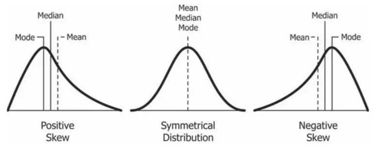
It measures the asymmetry of a data distribution.
Tells us whether the data is concentrated on one side of mean and is there a long tail stretching on the other side.
Positive Skew:
- Tail is longer on the right side of the mean.
- Bulk of data is on the left side of the mean, but there are a few very high values pulling the mean towards the right.
- Mean > Median > Mode.
Negative Skew:
- Tail is longer on the left side of the mean.
- Bulk of data is on the right side of the mean, but there are a few very high values pulling the mean towards the left.
- Mean < Median < Mode.
Zero Skew:
- Perfectly symmetrical like a normal distribution.
- Mean = Median = Mode.
- Consider the salary of employees in a company. Most employees earn a very modest salary, but a few executives earn
extremely high salaries. This dataset will be positively skewed with the mean salary > median salary.
Median salary would be a better representation of the typical salary of employees.
It measures the “tailedness” of a data distribution.
It describes how much the data is concentrated in tails (fat or thin) versus the center.
- It can tell us about the frequency of outliers in the data.
- Thick tails => More outliers.
Excess Kurtosis:
Excess kurtosis is calculated by subtracting 3 from standard kurtosis in order to compare with normal distribution.
Normal distribution has kurtosis = 3.
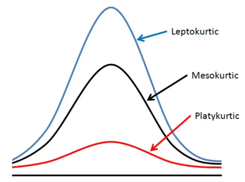
Mesokurtic:
- Excess kurtosis = 0 i.e normal kurtosis.
- Tails are neither too thick nor too thin.
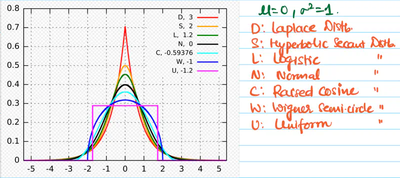
Leptokurtic:
- High kurtosis, i.e, excess kurtosis > 0 (+ve).
- Heavy or thick tails => High probability of outliers.
- Sharp peak => High concentration of data around mean.
- E.g: Student’s t-distribution, Laplace distribution, etc.
- High risk stock portfolios.
Platykurtic:
- Low kurtosis, i.e, excess kurtosis < 0 (-ve).
- Thin tails => Low probability of outliers.
- Low peak => more uniform distribution of values.
- E.g: Uniform distribution, Bernoulli(P=0.5) distribution, etc.
- Investment in fixed deposits.
E.g: Percentile, Quartile, Inter Quartile Range(IQR), etc.
It indicates the percentage of scores in a dataset that are equal to or below a specific value.
Here, the complete dataset is divided into 100 equal parts.
- \(k^{th}\) percentile => at least \(k\) percent of the data points are equal to or below the value.
- It is a relative comparison, i.e, compares a score with the entire group’s performance.
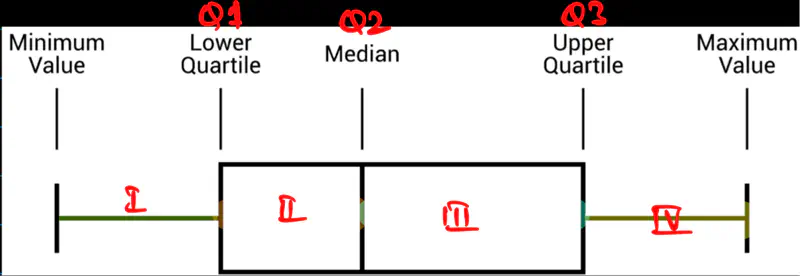
- Quartiles are basis for box plots.
- 90th percentile => score is higher than 90% of of all other test takers.
They are special percentiles that divide the complete dataset into 4 equal parts.
Q1 => 25th percentile, value below which 25% of the data falls.
Q2 => 50th percentile, value below which 50% of the data falls; median.
Q3 => 75th percentile, value below which 75% of the data falls.
- Data = \(\{1,2,3,4,5,6,7,8,9,10,100\}\) \[ Q1 = (11+1) * 1/4 = 12*1/4 = 3 \\ Q2 = (11+1) * 1/2 = 12*1/2 = 6 \\ Q3 = (11+1) * 3/4 = 12*3/4 = 9 \]
It is the single number that measures the spread of middle 50% of the data, i.e Q1-Q3.
- More robust measure of spread than range as is NOT impacted by outliers.
IQR = Q3 - Q1
- Data = \(\{1,2,3,4,5,6,7,8,9,10,100\}\) \[ Q1 = (11+1) * 1/4 = 12*1/4 = 3 \\ Q2 = (11+1) * 1/2 = 12*1/2 = 6 \\ Q3 = (11+1) * 3/4 = 12*3/4 = 9 \]
Therefore, IQR = Q3-Q1 = 9-3 = 6
IQR is a standard tool for detecting outliers.
Values that fall outside the ‘fences’ can be considered as potential outliers.
Lower fence = Q1 - 1.5 * IQR
Upper fence = Q3 + 1.5 * IQR
- Data = \(\{1,2,3,4,5,6,7,8,9,10,100\}\) \[ Q1 = (11+1) * 1/4 = 12*1/4 = 3 \\ Q2 = (11+1) * 1/2 = 12*1/2 = 6 \\ Q3 = (11+1) * 3/4 = 12*3/4 = 9 \]
IQR = Q3-Q1 = 9-3 = 6
Lower fence = Q1 - 1.5 * IQR = 3 - 9 = -6
Upper fence = Q3 + 1.5 * IQR = 9 + 9 = 18
So, any data point that is less than -6 or greater than 18 is considered as a potential outlier.
As in this example, 100 can be considered as an outlier.
Even though the above metrics give us a good idea of the data distribution,
but still we should always plot the data and visually inspect the data distribution.
As these metrics may not provide the complete picture.
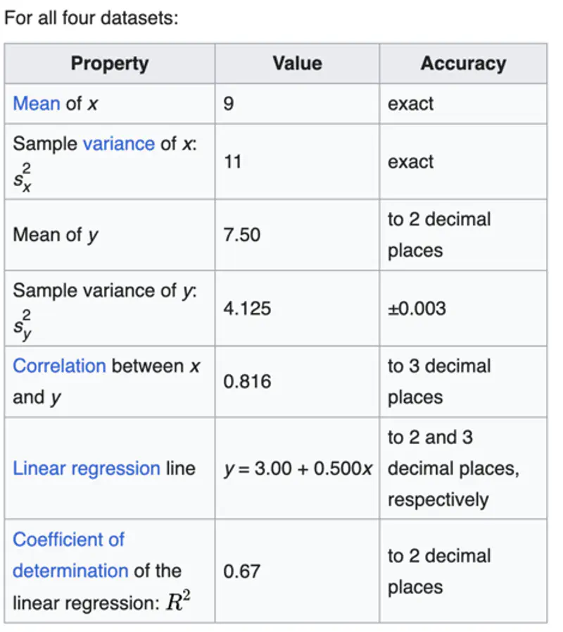
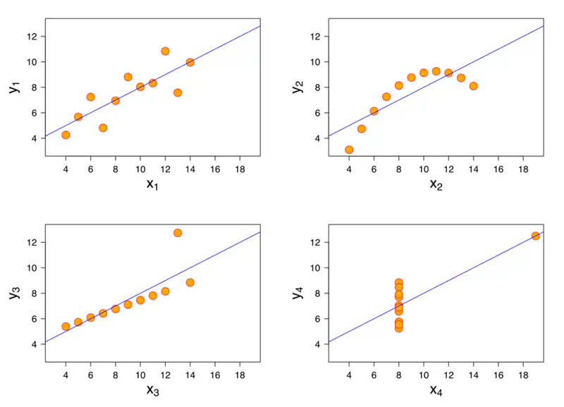
A mathematician called Francis John Anscombe has illustrated this point beautifully in his Anscombe’s Quartet.
Anscombe’s quartet:
It comprises four datasets that have nearly identical simple descriptive statistics,
yet have very different distributions and appear very different when plotted.
End of Section
2.2 - Correlation
It measures the direction of linear relationship between two variables \(X\) and \(Y\).
\(N\) = size of population
\(\mu_{x}\) = population mean of \(X\)
\(\mu_{y}\) = population mean of \(Y\)
\(n\) = size of sample
\(\bar{x}\) = sample mean of \(X\)
\(\bar{y}\) = sample mean of \(Y\)
Note: We have a term (n-1) instead of n in the denominator to make it an unbiased estimate, called Bessel’s Correction.
If both \((x_i - \bar{x})\) and \((y_i - \bar{y})\) have the same sign, then the product is positive(+ve).
If both \((x_i - \bar{x})\) and \((y_i - \bar{y})\) have opposite signs, then the product is negative(-ve).
The final value of covariance depends on the sum of the above individual products.
\( \begin{aligned} \text{Cov}(X, Y) &> 0 &&\Rightarrow \text{ } X \text{ and } Y \text{ increase or decrease together} \\ \text{Cov}(X, Y) &= 0 &&\Rightarrow \text{ } \text{No linear relationship} \\ \text{Cov}(X, Y) &< 0 &&\Rightarrow \text{ } \text{If } X \text{ increases, } Y \text{ decreases (and vice versa)} \end{aligned} \)
Limitation:
Covariance is scale-dependent, i.e, units of X and Y impact its magnitude.
This makes it hard to make comparisons of covariance across different datasets.
E.g: Covariance between age and height will NOT be same as the covariance between years of experience and salary.
Note:It only measures the direction of the relationship, but does NOT give any information about the strength of the relationship.
- \(X = [1, 2, 3] \) and \(Y = [2, 4, 6] \)
Let’s calculate the covariance:
\(\text{Cov}(X, Y) = \frac{1}{n-1}\sum_{i=1}^{n}(x_i - \bar{x})(y_i - \bar{y})\)
\(\bar{x} = 2\) and \(\bar{y} = 4\)
\(\text{Cov}(X, Y) = \frac{1}{3-1}[(1-2)(2-4) + (2-2)(4-4) + (3-2)(6-4)]= 0\)
\( = \frac{1}{2}[2+0+2]= 2\)
=> Cov(X,Y) > 0 i.e if X increases, Y increases and vice versa.
It measures both the strength and direction of the linear relationship between two variables \(X\) and \(Y\).
It is a standardized version of covariance that gives a dimensionless measure of linear relationship.
There are 2 popular ways to calculate correlation coefficient:
- Pearson Correlation Coefficient (r)
- Spearman Rank Correlation Coefficient (\(\rho\))
It is a standardized version of covariance and most widely used measure of correlation.
Assumption: Data is normally distributed.
\(\sigma_{x}\) and \(\sigma_{y}\) are the standard deviations of \(X\) and \(Y\).
Range of \(r\) is between -1 and 1.
\(r = 1\) => perfect +ve linear relationship between X and Y
\(r = -1\) => perfect -ve linear relationship between X and Y
\(r = 0\) => NO linear relationship between X and Y.
Note: A correlation coefficient of 0.9 means that there is a strong linear relationship between X and Y,
irrespective of their units.
- \(X = [1, 2, 3] \) and \(Y = [2, 4, 6] \)
Let’s calculate the covariance:
\(\text{Cov}(X, Y) = \frac{1}{n-1}\sum_{i=1}^{n}(x_i - \bar{x})(y_i - \bar{y})\)
\(\bar{x} = 2\) and \(\bar{y} = 4\)
\(\text{Cov}(X, Y) = \frac{1}{3-1}[(1-2)(2-4) + (2-2)(4-4) + (3-2)(6-4)]= 0\)
\( => \text{Cov}(X, Y) = \frac{1}{2}[2+0+2]= 2\)
Let’s calculate the standard deviation of \(X\) and \(Y\):
\(\sigma_{x} = \sqrt{\frac{1}{n-1}\sum_{i=1}^{n}(x_i - \bar{x})^2} \)
\(= \sqrt{\frac{1}{3-1}[(1-2)^2 + (2-2)^2 + (3-2)^2]}\)
\(= \sqrt{\frac{1+0+1}{2}} =\sqrt{\frac{2}{2}} = 1 \)
Similarly, we can calculate the standard deviation of \(Y\):
\(\sigma_{y} = \sqrt{\frac{1}{n-1}\sum_{i=1}^{n}(y_i - \bar{y})^2} \)
\(= \sqrt{\frac{1}{3-1}[(2-4)^2 + (4-4)^2 + (6-4)^2]}\)
\(= \sqrt{\frac{4+0+4}{2}} =\sqrt{\frac{8}{2}} = 2 \)
Now, we can calulate the pearson correlation coefficient (r):
\(r_{xy} = \frac{Cov(X, Y)}{\sigma_{x} \sigma_{y}}\)
=> \(r_{xy} = \frac{2}{1* 2}\)
=> \(r_{xy} = 1\)
Therefore, we can say that there is a strong +ve linear relationship between X and Y.
It is a measure of the strength and direction of the monotonic relationship between two ranked variables \(X\) and \(Y\).
It captures monotonic relationship, meaning the variables move in the same or opposite direction,
but not necessarily a linear relationship.
- It is used when Pearson’s correlation is not suitable, such as, ordinal data, or when the continuous data does not meet the assumptions of linear methods, such as, Pearson’s correlation.
- Non-parametric measure of correlation that uses ranks instead of raw data.
- Quantifies how well the ranks of one variable predict the ranks of the other variable.
- Range of \(\rho\) is between -1 and 1.
- Compute the correlation of ranks awarded to a group of 5 students by 2 different teacherrs.
Student Teacher A Rank Teacher B Rank \(d_i\) \(d_i^2\) S1 1 2 -1 1 S2 2 1 1 1 S3 3 3 0 0 S4 4 5 -1 1 S5 5 4 1 1
\(\sum_{i}d_i^2 = 4 \)
\( n = 5 \)
\(\rho_{xy} = 1 - \frac{6\sum_{i}d_i^2}{n(n^2-1)}\)
=> \(\rho_{xy} = 1 - \frac{6*4}{5(5^2-1)}\)
=> \(\rho_{xy} = 1 - \frac{24}{5*24}\)
=> \(\rho_{xy} = 1 - \frac{1}{5}\)
=> \(\rho_{xy} = 0.8\)
Therefore, we can say that there is a strong +ve correlation between the ranks given by teacher A and teacher B.
- \(X = [1, 2, 3] \) and \(Y = [1, 8, 27] \)
Here, Spearman’s rank correlation coefficient \(\rho\) will be perfect 1 as there is a monotonic relationship i.e as X increases, Y increases and vice versa.
But, the Pearson’s correlation coefficient (r) will be slightly less than 1 i.e r = 0.9662.
Correlation is very useful in feature selection for training machine learning models.
- If 2 features are highly correlated => they provide redundant information.
- One of the features can be removed without significant loss of information.
- Keeping both can cause issues, such as, multicollinearity.
- If a feature is highly correlated with the target variable => this feature is a strong predictor, so keep it.
- A feature with very low or near zero correlation with the target variable may be considered for removal, as they have little predictive power.
Causation means that one variable directly causes the change in another variable, i.e, direct
cause->effect relationship.
Whereas, correlation means that two variables move together.
- Correlation does NOT imply Causation.
- Correlation simply shows an association between two variables that could be coincidental or due to some third, unobserved, factor.
E.g: Election results and stock market - there may be some correlation between the two,
but establishing clear causal links is difficult.
End of Section
2.3 - Central Limit Theorem
It is the true average of the entire group.
It describe the central tendency of the entire population.
\( \mu = \frac{1}{N}\sum_{i=1}^{N}x_i \)
N: Number of data points
It is the average of a smaller representative subset (a sample) of the entire population.
It provides an estimate of the population mean.
\( \bar{x} = \frac{1}{n}\sum_{i=1}^{n}x_i \)
n: size of sample
the sample mean converges to the true the population mean.
In other words, a long-run average of a repeated random variable approaches the expected value.
This law states that for a sequence of of I.I.D random variables \( X_1, X_2, \dots, X_n \),
with finite mean and variance, the distribution of the sample mean \( \bar{X} \) approaches a normal distribution
as \( n \rightarrow \infty \), regardless of its original population distribution.
The distribution of the sample mean is : \( \bar{X} \sim N(\mu, \sigma^2/n)\)
Let, \( X_1, X_2, \dots, X_n \) are I.I.D random variables.
- Population mean = \(E[X_i] = \mu < \infty\)
- Population Variance = \(Var[X_i] = \sigma^2 < \infty \)
- Sample mean = \( \bar{X_n} = \frac{1}{n}\sum_{i=1}^{n}X_i = \frac{1}{n}(X_1 + X_2+ \dots +X_n) \)
- Variance of sample means = \( Var[\bar{X_n}] = Var[\frac{1}{n}(X_1+ X_2+ \dots+ X_n)]\)
Now, let’s calculate the variance of sample means.
We know that:
- \(Var[X+Y] = Var[X] + Var[Y] \), for independent random variables X and Y.
- \(Var[cX] = c^2Var[X] \), for constant ‘c’.
Let’s apply above 2 rules on the variance of sample means equation above:
\[ \begin{aligned} Var[\bar{X_n}] &= Var[\frac{1}{n}(X_1+ X_2+ \dots+ X_n)] \\ &= \frac{1}{n^2}[Var[X_1+ X_2+ \dots+ X_n]] \\ &= \frac{1}{n^2}[Var[X_1] + Var[X_2] + \dots + Var[X_n]] \\ \text{We know that: } Var[X_i] = \sigma^2 \\ &= \frac{1}{n^2}[\sigma^2 + \sigma^2 + \dots + \sigma^2] \\ &= \frac{n\sigma^2}{n^2} \\ => Var[\bar{X_n}] &= \frac{\sigma^2}{n} \end{aligned} \]Since, standard deviation = \(\sigma = \sqrt{Variance}\)
Therefore, Standard Deviation\([\bar{X_n}] = \sqrt{\frac{\sigma^2}{n}} = \frac{\sigma}{\sqrt{n}}\)
The standard deviation of the sample means is also known as “Standard Error”.
Note: We can also standardize the sample mean, i.e, mean centering and variance scaling.
Standardisation helps us to use the Z-tables of normal distribution.
We know that, a standardized random variable \(Y_i = \frac{X_i - \mu}{\sigma}\)
Similarly, standardized sample mean:
Note: For practical purposes, \(n \ge 30\) is considered as a sufficient sample size for the CLT to hold.
- Let’s collect the data for height of people in a city to find the average height of people in the city.
- Sample size (n) = 100
- And then repeat this data collection process 1000 times.
- For each of these 1000 (k) samples, calculate the sample mean \(X_1, X_2, \dots, X_{1000(k)} \)
- Now, when we plot these 1000(k) sample means, the resulting distribution will be very close to a normal/Gaussian distribution.
\(\bar{X_n} \sim N(\mu, \sigma^2/n)\), for large n, typically \(n \ge 30\).
Note:
- ‘k’ = a large number of repetitions allows us to observe the distribution of sample means after plotting.
- ’n’ = number of samples in each repetition is fixed for any given calculation of sample mean \(\bar{X_n}\).
The variance must be finite, else, the sample mean will NOT converge to a normal distribution.
If a distribution has a heavy tail, then the expected value calculation diverges.
e.g:
- Cauchy distribution has infinite mean and infinite variance.
- Pareto distribution (with low alpha) has infinite variance, such as distribution of wealth.
End of Section
2.4 - Confidence Interval
It is a range of values that is likely to contain the true population mean, based on a sample.
Instead of giving a point estimate, it gives a range of values with confidence level.
For normal distribution, confidence interval :
\(\bar{X}\): Sample mean
\(Z\): Z-score corresponding to confidence level
\(n\): Sample size
\( \sigma \): Population Standard Deviation
Applications:
- A/B testing, i.e., compare 2 or more versions of a product.
- ML model performance evaluation, i.e, instead of giving a single performance score of say 85%,
it is better to provide a 95% confidence interval, such as, [82.5%, 87.8%].
95% confidence interval does NOT mean there is a 95% chance that the true mean lies in the specific calculated interval.
- It just means that if we repeat the sampling process many times, then 95% of of those calculated intervals will capture or contain the true population mean \(\mu\).
- Also, we cannot say there is 95% probability that the true mean is within that specific range because true population mean is a fixed constant, NOT a random variable.
Let’s suppose we want to measure the average weight of a certain species of dog.
We want to estimate the true population
mean \(\mu\) using confidence interval.
Note: True average weight = 30 kg, but this is NOT known to us.
| Sample Number | Sample Mean | 95% Confidence Interval | Did it capture \(\mu\) ? |
|---|---|---|---|
| 1 | 29.8 kg | (28.5, 31.1) | Yes |
| 2 | 30.4 kg | (29.1, 31.7) | Yes |
| 3 | 31.5 kg | (30.2, 32.8) | No |
| 4 | 28.1 kg | (26.7, 29.3) | No |
| - | - | - | - |
| - | - | - | - |
| - | - | - | - |
| 100 | 29.9 kg | (28.6, 31.2) | Yes |
- We generated 100 confidence intervals(CI) each based on different samples.
- 95% CI guarantees that, in long run, 95 out of 100 CIs will include the true average weight, i.e, \(\mu=30kg\), and may be will miss 5 out of 100 times.
Suggest which company is offering a better salary?
Below is the details of the salaries based on a survey of 50 employees.
| Company | Average Salary(INR) | Standard Deviation |
|---|---|---|
| A | 36 lpa | 7 lpa |
| B | 40 lpa | 14 lpa |
For comparison, let’s calculate the 95% confidence interval for the average salaries of both companies A and B.
We know that:
\( CI = \bar{X} \pm Z\frac{\sigma}{\sqrt{n}} \)
Margin of Error(MoE) \( = Z\frac{\sigma}{\sqrt{n}} \)
Z-Score for 95% CI = 1.96
\(MoE_A = 1.96*\frac{7}{\sqrt{50}} \approx 1.94 \)
=> 95% CI for A = \(36 \pm 1.94 \) = [34.06, 37.94]
\(MoE_B = 1.96*\frac{14}{\sqrt{50}} \approx 3.88\)
=> 95% CI for B = \(40 \pm 3.88 \) = [36.12, 43.88]
We can see that initially company B’s salary looked obviously better,
but after calculating the 95% CI, we can see that there is a significant overlap in the salaries of two companies,
i.e [36.12, 37.94].
End of Section
2.5 - Hypothesis Testing
Hypothesis Testing is used to determine whether a claim or theory about a population is supported by a sample data,
by assessing whether observed difference or patterns are likely due to chance or represent a true effect.
- It allows companies to test marketing campaigns or new strategies on a small scale before committing to larger investments.
- Based on the results of hypothesis testing, we can make reliable inferences about the whole group based on a representative sample.
- It helps us determine whether an observed result is statistically significant finding, or if it could have just happened by random chance.
It is a statistical inference framework used to make decisions about a population parameter, such as, the mean, variance,
distribution, correlation, etc., based on a sample of data.
It provides a formal method to evaluate competing claims.
Null Hypothesis (\(H_0\)):
Status quo or no-effect or no difference statement; almost always contains a statement of equality.
Alternative Hypothesis (\(H_1 ~or~ H_a\)):
The statement representing an effect, a difference, or a relationship.
It must be true if the null hypothesis is rejected.
- Test of Means:
- 1-Sample Mean Test: Compare sample mean to a known population mean.
- 2-Sample Mean Test: Compare means of 2 populations.
- Paired Mean Test: Compare means when data is paired, e.g., before vs. after test.
- Test of Median:
- Mood’s Median Test
- Sign Test
- Wilcoxon Signed Rank Test (non-parametric)
- Test of Variance:
- Chi-Square Test for a single variance
- F-Test to compare variances of 2 populations
- Test of Distribution(Goodness of Fit):
- Kolmogorov-Smirnov Test
- Shapiro-Wilk Test
- Anderson-Darling Test
- Chi-Square Goodness of Fit Test
- Test of Correlation:
- Pearson’s Correlation Coefficient Test
- Spearman’s Rank Correlation Test
- Kendall’s Tau Correlation Test
- Chi-Square Test of Independence
- Regression Test:
- T-Test: For regression coefficients
- F-Test: For overall regression significance
Step 1: Define the null and alternative hypotheses.
Step 2: Select a relevant statistical test for the task with associated test statistic.
Step 3: Calculate the test statistic under null hypothesis.
Step 4: Select a significance level (\(\alpha\)), i.e, the maximum acceptable false positive rate;
typically - 5% or 1%.
Step 5: Compute the p-value from the observed value of test-statistic.
Step 6: Make a decision to either accept or reject the null hypothesis, based on the significance level (\(\alpha\)).
Say, the data, D: <patient_id, med_1/med_2, recovery_time(in days)>
We need some metric to compare the recovery times of 2 medicines.
We can use the mean recovery time as the metric, because we know that we can use following techniques for comparison:
- 2-Sample T-Test; if \(n < 30\) and population standard deviation \(\sigma\) is unknown.
- 2-Sample Z-Test; if \(n \ge 30\) and population standard deviation \(\sigma\) is known.
Note: Let’s assume the sample size \(n < 30\), because medical tests usually have small sample sizes.
=> We will use the 2-Sample T-Test; we will continue using T-Test throughout the discussion.
Step 1: Define the null and alternative hypotheses.
Null Hypothesis \(H_0\): The mean recovery time of 2 medicines is the same i.e \(Mean_{m1} = Mean_{m2}\) or \(m_{m1} = m_{m2}\).
Alternate Hypothesis \(H_a\): \(m_{m1} < m_{m2}\) (1-Sided T-Test) or \(m_{m1} ⍯ m_{m2}\) (2-Sided T-Test).
Step 2: Select a relevant statistical test for the task with associated test statistic.
Let’s do a 2 sample T-Test, i.e, \(m_{m1} < m_{m2}\)
Step 3: Calculate the test statistic under null hypothesis.
Test Statistic:
For 2 sample T-Test:
s: Standard Deviation
n: Sample Size
Note: If the 2 means are very close then \(t_{obs} \approx 0\).
Step 4: Suppose significance level (\(\alpha\)) = 5% or 0.05.
Step 5: Compute the p-value from the observed value of test-statistic.
P-Value:
p-value = area under curve = probability of observing test statistic \( \ge t_{obs} \) if the null hypothesis is true.
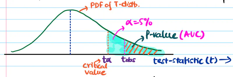
Step 6: Accept or reject the null hypothesis, based on the significance level (\(\alpha\)).
If \(p_{value} < \alpha\), we reject the null hypothesis and accept the alternative hypothesis and vice versa.
Note: In the above example \(p_{value} < \alpha\), so we reject the null hypothesis.
We need to do a left or right sided test, or a 2-sided test, this depends upon our alternate hypothesis and test statistic.
Let’s continue our 2 sample mean T-test to understand the concept:
Left Sided/Tailed Test:
\(H_a\): Mean recovery time of medicine 1 < medicine 2, i.e, \(m_{m_1} < m_{m_2}\)
=> \(m_{m_1} - m_{m_2} < 0\)
Since, the denominator in above equation is always positive.
=> \(t_{obs} < 0\)
Therefore, we need to do a left sided/tailed test.
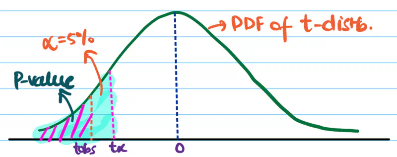
So, we want \(t_{obs}\) to be very negative to confidently conclude that alternate hypothesis is true.
Right Sided/Tailed Test:
\(H_a\): Mean recovery time of medicine 1 > medicine 2, i.e, \(m_{m_1} > m_{m_2}\)
=> \(m_{m_1} - m_{m_2} > 0\)
Similarly, here we need to do a right sided/tailed test.
2 Sided/Tailed Test:
\(H_a\): Mean recovery time of medicine 1 ⍯ medicine 2, i.e, \(m_{m_1} ⍯ ~ m_{m_2}\)
=> \(m_{m_1} - m_{m_2} < 0\) or \(m_{m_1} - m_{m_2} > 0\)
If \(H_a\) is true then \(t_{obs}\) is a large -ve value or a large +ve value.
Since, t-distribution is symmetric, we can divide the significance level \(\alpha\) into 2 equal parts.
i.e \(\alpha = 2.5\%\) on each side.
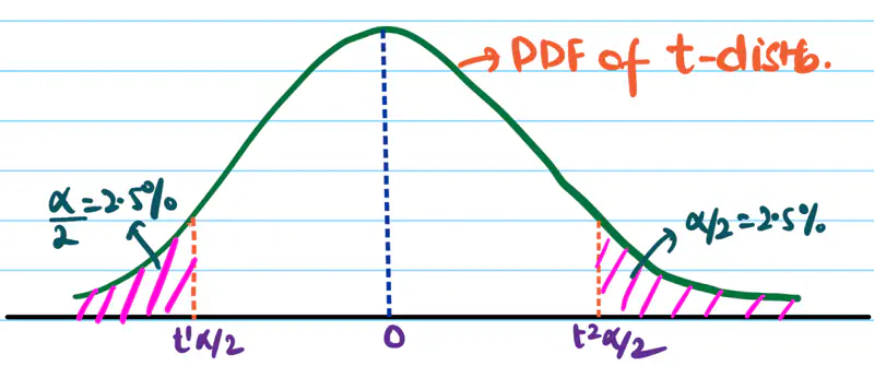
So, we want \(t_{obs}\) to be very negative or very positive to confidently conclude that the alternate hypothesis is true. We accept \(H_a\) if \(t_{obs} < t^1_{\alpha/2}\) or \(t_{obs} > t^2_{\alpha/2}\).
Note: For critical applications ‘\(\alpha\)’ can be very small i.e. 0.1% or 0.01%, e.g medicine.
It is the probability of wrongly rejecting a true null hypothesis, known as a Type I error or false +ve rate.
- Tolerance level of wrongly accepting alternate hypothesis.
- If the p-value < \(\alpha\), we reject the null hypothesis and conclude that the finding is statistically NOT so significant..
It is a specific point on the test-statistic distribution that defines the boundaries of the null hypothesis
acceptance/rejection region.
It tells us that at what value (\(t_{\alpha}\)) of test statistic will the area under curve be equal to the significance level \(\alpha\).
For a right tailed/sided test:
- if \(t_{obs} > t_{\alpha} => p_{value} < \alpha\); therefore, reject null hypothesis.
- if \(t_{obs} < t_{\alpha} => p_{value} \ge \alpha\); therefore, failed to reject null hypothesis.
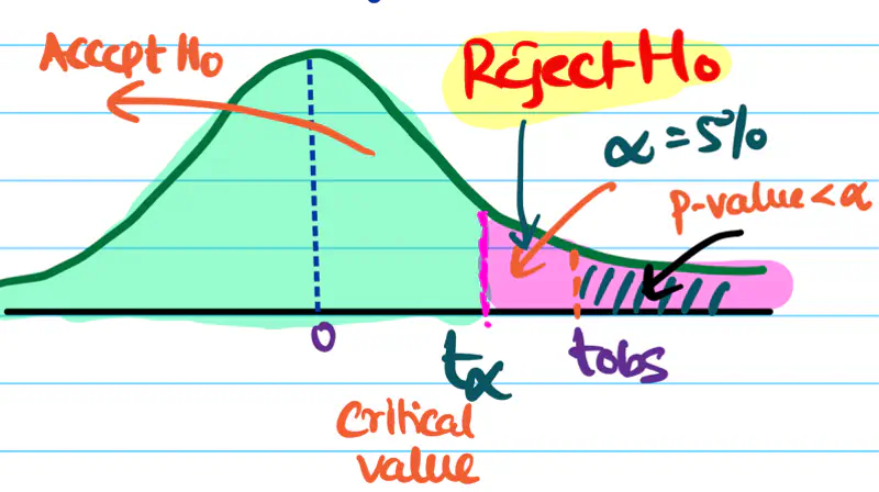
It is the probability that a hypothesis test will correctly reject a false null hypothesis (\(H_{0}\)) when the alternative hypothesis (\(H_{a}\)) is true.
Power of test = \(1 - \beta\)
Probability of correctly accepting alternate hypothesis (\(H_{a}\))
\(\alpha\): Probability of wrongly accepting alternate hypothesis \(H_{a}\)
\(\beta\): Probability of wrongly rejecting alternate hypothesis \(H_{a}\)
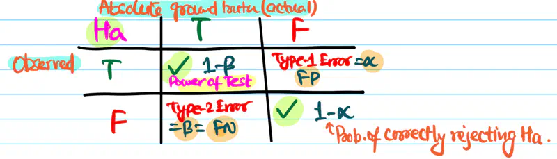
Yes, having a large sample size makes a hypothesis test more powerful.
- As n increases, sample mean \(\bar{x}\) approaches the population mean \(\mu\).
- Also, as n increases, t-distribution approaches normal distribution.
It is a standardized objective measure that complements p-value by clarifying whether a statistically significant
finding has any real world relevance.
It quantifies the magnitude of relationship between two variables.
- Larger effect size => more impactful effect.
- Standardized (mean centered + variance scaled) measure allows us to compare the imporance of effect across various studies or groups, even with different sample sizes.
Effect size is measured using Cohen’s d formula:
\(\bar{X}\): Sample mean
\(s_p\): Pooled Standard deviation
\(n\): Sample size
\(s\): Standard deviation
Note: Theoretically, Cohen’s d value can range from negative infinity to positive infinity.
but for practical purposes, we use the following value:
small effect (\(d=0.2\)), medium effect (\(d=0.5\)), and large effect (\(d\ge 0.8\)).
More overlap => less effect i.e low Cohen’s d value.
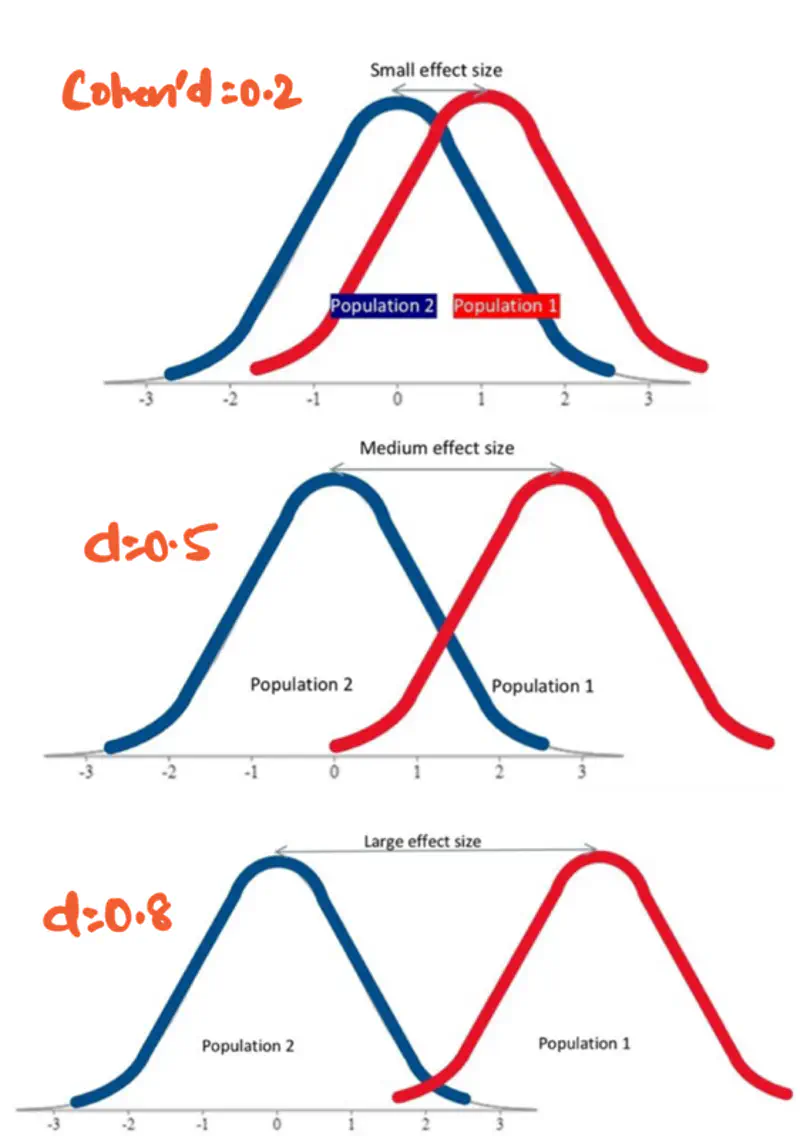
- A study on drug trials finds that patients taking a new drug had statistically significant
improvement (p-value<0.05), compared to a placebo group.
- Small effect size: Cohen’s d = 0.1 => drug had minimal effect.
- Large effect size: Cohen’s d = 0.8 => drug produced substantial improvement.
End of Section
2.6 - T-Test
It is a statistical test that is used to determine whether the sample mean is equal to a hypothesized value or
is there a significant difference between the sample means of 2 groups.
- It is a parametric test, since it assumes data to be approximately normally distributed.
- Appropriate when:
- sample size n < 30.
- population standard deviation \(\sigma\) is unknown.
- It is based on Student’s t-distribution.
It is a continuous probability distribution that is a symmetrical, bell-shaped curve similar
to the normal distribution but with heavier tails.
Shape of the curve or mass in tail is controlled by degrees of freedom.
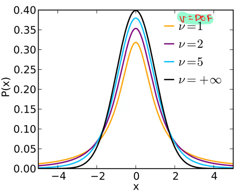
There are 3 types of T-Test:
- 1-Sample T-Test: Test if sample mean differs from hypothesized value.
- 2-Sample T-Test: Test whether there is a significant difference between the means of two independent groups.
- Paired T-Test: Test whether 2 related samples differ, e.g., before and after.
Generally speaking, it represents the number of independent values that are free to vary in a dataset when estimating a parameter.
e.g.: If we have k observations and their sum = 50.
The sum of (k-1) terms can be anything, but the kth term is fixed at 50 - (sum of other (k-1) terms).
So, we have only (k-1) terms that can change independently, therefore, the DOF(\(\nu\)) = k-1.
It is used to test whether the sample mean is equal to a known/hypothesized value.
Test statistic (t):
where,
\(\bar{x}\): sample mean
\(\mu\): hypothesized value
\(s\): sample standard deviation
\(n\): sample size
\(\nu = n-1 \): degrees of freedom
Tester ran the test 20 times and found the average API repsonse time to be 115 ms, with a standard deviation of 25 ms.
Is the developer’s claim valid?
Let’s verify developer’s claim using the tester’s test results using 1 sample t-test.
Null hypothesis: \(H_0\) = The average API response time is 100 ms, i.e, \(\bar{x} = \mu\).
Alternative hypothesis: \(H_a\) = The average API response time > 100 ms, i.e, \(\bar{x} > \mu\) => right tailed test.
Hypothesized mean \(\mu\) = 100 ms
Sample mean \(\bar{x}\) = 115 ms
Sample standard deviation \(s\) = 25 ms
Sample size \(n\) = 20
Degrees of freedom \(\nu\) = 19
\( t_{obs} = \frac{\bar{x} - \mu}{s/\sqrt{n}}\) = \(\frac{115 - 100}{25/\sqrt{20}}\)
= \(\frac{15\sqrt{20}}{25} = \frac{3\sqrt{20}}{5} \approx 2.68\)
Let significance level \(\alpha\) = 5% =0.05.
Critical value \(t_{0.05}\) = 1.729
Important: Find the value of \(t_{\alpha}\) in T-table
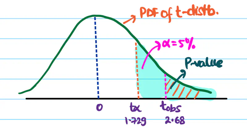
Since \(t_{obs}\) > \(t_{0.05}\), we reject the null hypothesis.
And, accept the alternative hypothesis that the API response time is significantly > 100 ms.
Hence, the developer’s claim is NOT valid.
It is used to determine whether there is a significant difference between the means of two independent groups.
There are 2 types of 2-sample t-test:
- Unequal Variance
- Equal Variance
Unequal Variance:
In this case, the variance of 2 independent groups is not equal.
Also called, Welch’s t-test.
Test statistic (t):
Equal Variance:
In this case, both samples come from equal or approximately equal variance.
Test statistic (t):
Here, degrees of freedom (for equal variance) \(\nu\) = \(n_1 + n_2 - 2\).
\(\bar{x}\): sample mean
\(s\): sample standard deviation
\(n\): sample size
\(\nu\): degrees of freedom
The AI team wants to validate whether the new ML model accuracy is better than the existing model’s accuracy.
Below is the data for the existing model and the new model.
| New Model (A) | Existing Model (B) | |
|---|---|---|
| Sample size (n) | 24 | 18 |
| Sample mean (\(\bar{x}\)) | 91% | 88% |
| Sample std. dev. (s) | 4% | 3% |
Given that the variance of accuracy scores of new and existing models are almost same.
Now, let’s follow our hypothesis testing framework.
Null hypothesis: \(H_0\): The accuracy of new model is same as the accuracy of existing model.
Alternative hypothesis: \(H_a\): The new model’s accuracy is better/greater than the existing model’s accuracy => right tailed test
Let’s solve this using 2 sample T-Test, since the sample size n < 30.
Since the variance of 2 sample are almost equal then we can use the pooled variance method.
Next let’s compute the test statistic, under null hypothesis.
DOF \(\nu\) = \(24+18-2\) = 42 - 2 = 40
Let significance level \(\alpha\) = 5% =0.05.
Critical value \(t_{0.05}\) = 1.684
Important: Find the value of \(t_{\alpha}\) in T-table
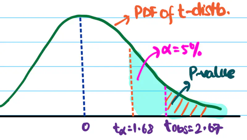
Since \(t_{obs}\) > \(t_{0.05}\), we reject the null hypothesis.
And, accept the alternative hypothesis that the new model has better accuracy than the existing model.
End of Section
2.7 - Z-Test
It is a statistical test used to determine whether there is a significant difference between mean of 2 groups or sample and population mean.
- It is a parametric test, since it assumes data to be normally distributed.
- Appropriate when:
- sample size \(n \ge 30\).
- population standard deviation \(\sigma \) is known.
- It is based on Gaussian/normal distribution.
- It compares the difference between means relative to standard error, i.e, standard deviation of sampling distribution of sample mean.
There are 2 types of Z-Test:
- 1-Sample Z-Test: Used to compare the mean of a sample mean with a population mean.
- 2-Sample Z-Test: Used to compare the sample means of 2 independent samples.
It is a standardized score that measures how many standard deviations a particular data point is away from the population mean \(\mu\).
- Transform a normal distribution \(\mathcal{N}(\mu, \sigma^2)\) to a standard normal distribution \(Z \sim \mathcal{N}(0, 1)\).
- Standardized score helps us compare values from different normal distributions.
Z-score is calculated as:
\[Z = \frac{x - \mu}{\sigma}\]x: data point
\(\mu\): population mean
\(\sigma\): population standard deviation
e.g:
- Z-score of 1.5 => data point is 1.5 standard deviations above the mean.
- Z-score of -2.0 => data point is 2.0 standard deviations below the mean.
Z-score helps to define probability areas:
- 68% of the data points fall within \(\pm 1 \sigma\).
- 95% of the data points fall within \(\pm 2 \sigma\).
- 99.7% of the data points fall within \(\pm 3 \sigma\).
Note:
- Z-Test applies the concept of Z-score to sample mean rather than a single data point.
It is used to test whether the sample mean \(\bar{x}\) is significantly different from a known population mean \(\mu\).
Test Statistic:
\(\bar{x}\): sample mean
\(\mu\): hypothesized population mean
\(\sigma\): population standard deviation
\(n\): sample size
\(\sigma / \sqrt{n}\): standard error of mean
Read more about Standard Error
Note: Test statistic Z follows a standard normal distribution \(Z \sim \mathcal{N}(0, 1)\).
It is used to test whether the sample means \(\bar{x_1}\) and \(\bar{x_2}\) of 2 independent samples are significantly different from each other.
Test Statistic:
\(\bar{x_1}\): sample mean of first sample
\(\bar{x_2}\): sample mean of second sample
\(\sigma_1\): population standard deviation of first sample
\(\sigma_2\): population standard deviation of second sample
\(n_1\): sample size of first sample
\(n_2\): sample size of second sample
Note: Test statistic Z follows a standard normal distribution \(Z \sim \mathcal{N}(0, 1)\).
After applying a new optimisation, and n=100 runs, yields a sample mean of 117 seconds.
Does the optimisation significantly reduce the runtime of the model?
Consider the significance level of 5%.
Null Hypothesis: \(\mu = 120\) seconds, i.e, no change.
Alternative Hypothesis: \(\mu < 120\) seconds => left tailed test.
We will use 1-sample Z-Test to test the hypothesis.
Test Statistic:
Since, significance level \(\alpha\) = 5% =0.05.
Critical value \(Z_{0.05}\) = -1.645
Important: Find the value of \(Z_{\alpha}\) in Z-Score Table
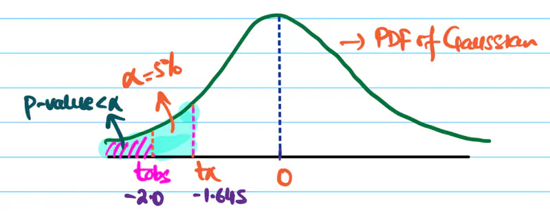
Our \(t_{obs}\) is much more extreme than the the critical value \(Z_{0.05}\), => p-value < 5%.
Hence, we reject the null hypothesis.
Therefore, there is a statistically significant evidence that the new optimisation reduces the runtime of the model.
It is a statistical hypothesis test used to determine if there is a significant difference between the proportion
of a characteristic in two independent samples or to compare a sample proportion to a known population value
- It is used when dealing with categorical data, such as, success/failure, male/female, yes/no etc.
It is of 2 types:
- 1-Sample Z-Test of Proportion: Used to test whether the observed proportion in a sample differs from hypothesized proportion.
- 2-Sample Z-Test of Proportion: Used to compare whether the 2 independent samples differ in their proportions.
The categorical data,i.e success/failure, is discrete that can be modeled as Bernoulli distribution.
Let’s understand how this Bernoulli random variable can be approximated as a Gaussian distribution for a very large sample size,
using Central Limit Theorem.
Read more about Central Limit Theorem
Note:We will not prove the complete thing, but we will understand the concept in enough depth for clarity.
\(Y \sim Bernoulli(p)\)
\(X \sim Binomial(n,p)\)
E[X] = mean = np
Var[X] = variance = np(1-p)
X = total number of successes
p = true probability of success
n = number of trials
Proportion of Success in sample = Sample Proportion = \(\hat{p} = \frac{X}{n}\)
e.g.: If n=100 people were surveyed, and 40 said yes, then \(\hat{p} = \frac{40}{100} = 0.4\)
By Central Limit Theorem, we can state that for very large ’n’ Binomial distribution’s mean and variance can be used as an
approximation for Gaussian/Normal distribution:
Since, \(\hat{p} = \frac{X}{n}\)
We can say that:
Mean = \(\mu_{\hat{p}} = p\) = True proportion of success in the entire population
Standard Error = \(SE_{\hat{p}} = \sqrt{Var[\frac{X}{n}]} = \sqrt{\frac{p(1-p)}{n}}\) = Standard Deviation of the sample proportion
Note: Large Sample Condition - Approximation is only valid when the expected number of successes and failures are both > 10 (sometimes 5).
\(np \ge 10 ~and~ n(1-p) \ge 10\)
It is used to test whether the observed proportion in a sample differs from hypothesized proportion.
\(\hat{p} = \frac{X}{n}\): Proportion of success observed in a sample
\(p_0\): Specific propotion value under the null hypothesis
\(SE_0\): Standard error of sample proportion under the null hypothesis
Z-Statistic: Measures how many standard errors is the observed sample proportion \(\hat{p}\) away from \(p_0\)
Test Statistic:
It is used to compare whether the 2 independent samples differ in their proportions.
- Standard test used in A/B testing.
A company wants to compare its 2 different website designs A & B.
Below is the table that shows the data:
| Design | # of visitors(n) | # of signups(x) | conversion rate(\(\hat{p} = \frac{x}{n}\)) |
|---|---|---|---|
| A | 1000 | 80 | 0.08 |
| B | 1200 | 114 | 0.095 |
Is the design B better, i.e, design B increases conversion rate or proportion of visitors who sign up?
Consider the significance level of 5%.
Null Hypothesis: \(\hat{p_A} = \hat{p_B}\), i.e, no difference in conversion rates of 2 designs A & B.
Alternative Hypothesis: \(\hat{p_B} > \hat{p_A}\) i.e conversion rate of B > A => right tailed test.
Check large sample condition for both samples A & B.
\(n\hat{p_A} = 80 > 10 ~and~ n(1-\hat{p_A}) = 920 > 10\)
Similarly, we can show for B too.
Pooled proportion:
\[ \bar{p} = \frac{x_A+x_B}{n_A+n_B} = \frac{80+114}{1000+1200} = \frac{194}{2200} \\[10pt] => \bar{p}\approx 0.0882 \]Standard Error(Pooled):
\[ SE=\sqrt{\bar{p}(1-\bar{p})(\frac{1}{n_1} +\frac{1}{n_2})} \\[10pt] = \sqrt{0.0882(1-0.0882)(\frac{1}{1000} +\frac{1}{1200})} \\[10pt] => SE \approx 0.0123 \]Test Statistic(Z):
\[ t_{obs} = \frac{\hat{p_B}-\hat{p_A}}{SE_{\hat{p_A}-\hat{p_B}}} \\[10pt] = \frac{0.095-0.0882}{0.0123} \\[10pt] => t_{obs} \approx 1.22 \]Significance level \(\alpha\) = 5% =0.05.
Critical value \(Z_{0.05}\) = 1.645
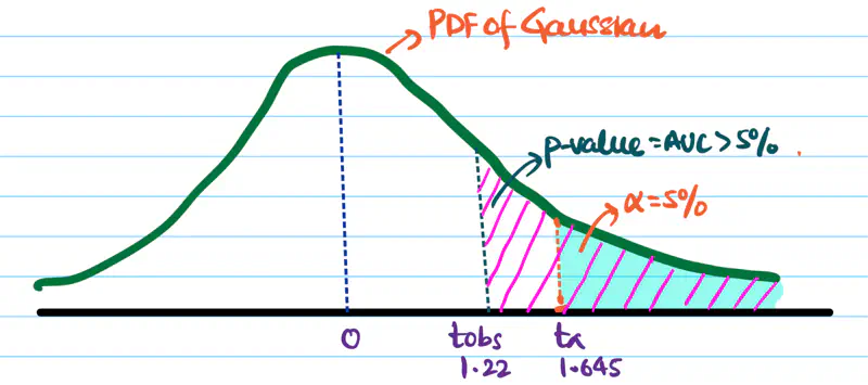
Since, \(t_{obs} < Z_{0.05}\) => p-value > 5%.
Hence, we fail to reject the null hypothesis.
Therefore, the observed conversion rate of design B is due to random chance; thus, B is not a better design.
End of Section
2.8 - Chi-Square Test
A random variable Q is said to follow a chi-square distribution with ’n’ degrees of freedom,i.e \(\chi^2(n)\),
if it is the sum of squares of ’n’ independent random variables that follow a standard normal distribution, i.e, \(N(0,1)\).
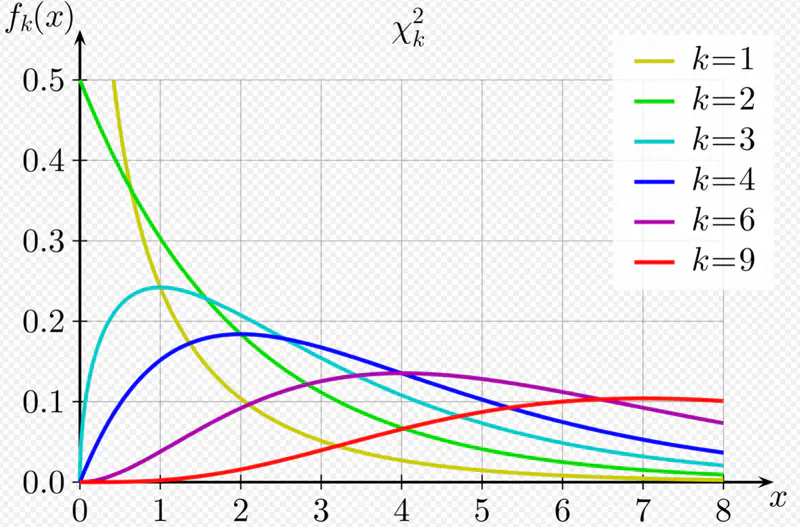
Key Properties:
- Non-negative, since sum of squares.
- Asymmetric, right skewed.
- Shape depends on the degrees of freedom; as \(\nu\) increases, the distribution becomes more symmetric and approaches a normal distribution.
Generally speaking, it represents the number of independent values that are free to vary in a dataset when estimating a parameter.
e.g.: If we have k observations and their sum = 50.
The sum of (k-1) terms can be anything, but the kth term is fixed at 50 - (sum of other (k-1) terms).
So, we have only (k-1) terms that can change independently, therefore, the DOF(\(\nu\)) = k-1.
More broadly, we can also say that sum/count of independent random variables approaches a normal distribution as the sample size increases.
Since, sample mean \(\bar{x} = \frac{sum}{n} \).
Read more about Central Limit Theorem
Note: We are dealing with categorical data, where there is a count associated with each category.
In the context of categorical data, the counts \(O_i\) are governed by multinomial distribution
(a generalisation of binomial distribution).
Multinomial distribution is defined for multiple classes or categories, ‘k’, and multiple trials ’n’.
For \(i^{th}\) category:
Probability of \(i^{th}\) category = \(p_i\)
Mean = Expected count/frequency = \(E_i = np_i \)
Variance = \(Var_i = np_i(1-p_i) \)
By Central Limit Theorem, for very large n, i.e, as \(n \rightarrow \infty\), the multinomial distribution can be approximated as a normal distribution.
The multinomial distribution of count/frequency can be approximated as :
\(O_i \approx N(np_i, np_i(1-p_i))\)
Standardized count (mean centered and variance scaled):
Under Null Hypothesis:
In Pearson’s proof of the chi-square test, the statistic is divided by the expected value (\(E_{i}\)) instead of the variance (\(Var_{i}\)),
because for count data that can be modeled using a Poisson distribution
(or a multinomial distribution where cell counts are approximately Poisson for large samples),
the variance is equal to the expected value (mean).
Therefore, \(Z_i \approx (O_{i}-E_{i})/\sqrt{E_{i}}\)
Note that the denominator is \(\sqrt{E_{i}}\) NOT \(\sqrt{Var_{i}}\).
\(O_{i}\): Observed count for \(i^{th}\) category
\(E_{i}\): Expected count for \(i^{th}\) category
Important: \(E_{i}\): Expected count should be large i.e >= 5 (typically) for a good enough approximation.
It is formed by squaring the approximately standard normal counts above, and summing them up.
For \(k\) categories, the test statistic is:
Note: For very large ’n’, the Pearson’s chi-square (\(\chi^2\)) test statistic follows a chi-square (\(\chi^2\)) distribution.
It is a non-parametric test for categorical data, i.e, does NOT make any assumption about the underlying distribution of the data, such as, normally distributed with known mean and variance; only uses observed and expected count/frequencies.
Note: Requires a large sample size.
It is used to compare the observed frequency distribution of a single categorical variable to a hypothesized or expected
probability distribution.
It can be used to determine whether a sample taken from a population follows a particular distribution,
e.g., uniform, normal, etc.
Test Statistic:
\(O_{i}\): Observed count for \(i^{th}\) category
\(E_{i}\): Expected count for \(i^{th}\) category, under null hypothesis \(H_0\)
\(k\): Number of categories
\(\nu\): Degrees of freedom = k - 1- m
\(m\): Number of parameters estimated from sample data to determine the expected probability
Note: Typical m=0, since, NO parameters are estimated.
- Kolmogorov-Smirnov (KS) Test: Compares empirical CDF with theoretical CDF of distribution.
- Anderson-Darling (AD) Test: Refinement of KS Test.
- Shapiro-Wilk (SW) Test: Specialised for normal distribution; good for small samples.
Find whether it is a fair coin (discrete uniform distribution test)?
Significance level = 5%
We need to find whether the coin is fair i.e we need to do a goodness of fit test for discrete uniform distribution.
Null Hypothesis \(H_0\): Coin is fair.
Alternative Hypothesis \(H_a\): Coin is biased towards head.
\(O_{H}\): Observed count head = 62
\(O_{T}\): Observed count head = 38
\(E_{i}\): Expected count for \(i^{th}\) category, under null hypothesis \(H_0\) = 50 i.e fair coin
\(k\): Number of categories = 2
\(\nu\): Degrees of freedom = k - 1- m = 2 - 1 - 0 = 1
Test Statistic:
Since, significance level = 5% = 0.05
Critical value = \(\chi^2(0.05,1)\) = 3.84
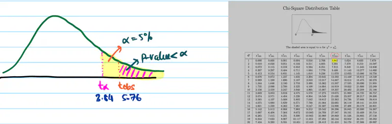
Since, \(t_{obs}\) = 5.76 > 3.84 (critical value), we reject the null hypothesis \(H_0\).
Therefore, the coin is biased towards head.
It is used to determine whether an association exists between two categorical variables,
using a contingency(dependency) table.
It is a non-parametric test, i.e, does NOT make any assumption about the underlying distribution of the data.
Test Statistic:
\(O_{ij}\): Observed count for \(cell_{i,j}\)
\(E_{ij}\): Expected count for \(cell_{i,j}\), under null hypothesis \(H_0\)
\(R\): Number of rows
\(C\): Number of columns
\(\nu\): Degrees of freedom = (R-1)*(C-1)
Let’s understand the above test statistic in more detail.
We know that, if 2 random variables A & B are independent, then,
\(P(A \cap B) = P(A, B) = P(A)*P(B)\)
i.e Joint Probability = Product of marginal probabilities.
Null Hypothesis \(H_0\): \(A\) and \(B\) are independent.
Alternative Hypothesis \(H_a\): \(A\) and \(B\) are dependent or associated.
N = Sample size
\(P(A_i) \approx \frac{Row ~~ Total_i}{N}\)
\(P(B_j) \approx \frac{Col ~~ Total_j}{N}\)
\(E_{ij}\) : Expected count for \(cell_{i,j}\) = \( N*P(A_i)*P(B_j)\)
=> \(E_{ij}\) = \(N*\frac{Row ~~ Total_i}{N}*\frac{Col ~~ Total_j}{N}\)
=> \(E_{ij}\) = \(\frac{Row ~~ Total_i * Col ~~ Total_j}{N}\)
\(O_{ij}\): Observed count for \(cell_{i,j}\)
A survey of 100 students was conducted to understand whether there is any relation between gender and beverage preference.
Below is the table that shows the number of students who prefer each beverage.
| Gender | Tea | Coffee | |
|---|---|---|---|
| Male | 20 | 30 | 50 |
| Female | 10 | 40 | 50 |
| 30 | 70 |
Significance level = 5%
Null Hypothesis \(H_0\): Gender and beverage preference are independent.
Alternative Hypothesis \(H_a\): Gender and beverage preference are dependent.
We know that Expected count for cell(i,j) = \(E_{ij}\) = \(\frac{Row ~~ Total_i * Col ~~ Total_j}{N}\)
\(E_{11} = \frac{50*30}{100} = 15\)
\(E_{12} = \frac{50*70}{100} = 35\)
\(E_{21} = \frac{50*30}{100} = 15\)
\(E_{22} = \frac{50*70}{100} = 35\)
Test Statistic:
Degrees of freedom = (R-1)(C-1) = (2-1)(2-1) = 1
Since, significance level = 5% = 0.05
Critical value = \(\chi^2(0.05,1)\) = 3.84
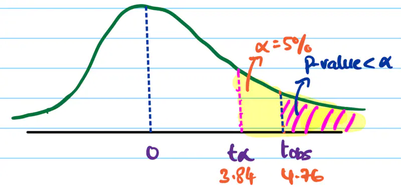
Since, \(t_{obs}\) = 4.76 > 3.84 (critical value), we reject the null hypothesis \(H_0\).
Therefore, the gender and beverage preference are dependent.
End of Section
2.9 - Performance Metrics
E.g.: For regression models, we have - MSE, RMSE, MAE, R^2 metric, etc.
Here, we will discuss various performance metrics for classification models.
It is a table that summarizes model’s predictions against the actual class labels, detailing where the model
succeeded and where it failed.
It is used for binary or multi-class classification problems.
| Predicted Positive | Predicted Negative | |
|---|---|---|
| Actual Positive | True Positive (TP) | False Negative (FN) |
| Actual Negative | False Positive (FP) | True Negative (TN) |
Type-1 Error:
It is the number of false positives.
e.g.: Model predicted that a patient has diabetes, but the patient actually does NOT have diabetes; “false alarm”.
Type-2 Error:
It is the number of false negatives.
e.g.: Model predicted that a patient does NOT have diabetes, but the patient actually has diabetes; “a miss”.
Many metrics are derived from the confusion matrix.
Precision:
It answers the question: “Of all the instances that the model predicted as positive, how many were actually positive?”
It measures exactness or quality of the positive predictions.
Recall:
It answers the question: “Of all the actual positive instances, how many did the model correctly identify?”
It measures completeness or coverage of the positive predictions.
F1 Score:
It is the harmonic mean of precision and recall.
It is used when we need a balance between precision and recall; also helpful when we have imbalanced data.
Harmonic mean penalizes extreme values more heavily, encouraging both metrics to be high.
| Precision | Recall | F1 Score | Mean |
|---|---|---|---|
| 0.5 | 0.5 | 0.50 | 0.5 |
| 0.7 | 0.3 | 0.42 | 0.5 |
| 0.9 | 0.1 | 0.18 | 0.5 |
Trade-Off:
Precision Focus:: Critical when cost of false positives is high.
e.g: Identify a potential terrorist.
A false positive, i.e, wrongly flagging an innocent person as a potential terrorist is very harmful.
Recall Focus:: Critical when cost of false negatives is high.
e.g.: Medical diagnosis of a serious disease.
A false negative, i.e, falsely missing a serious disease can cost someone’s life.
Analyze the performance of an access control system. Below is the data for 1000 access attempts.
| Predicted Authorised Access | Predicted Unauthorised Access | |
|---|---|---|
| Actual Authorised Access | 90 (TP) | 10 (FN) |
| Actual Unauthorised Access | 1 (FP) | 899 (TN) |
When the system allows access, it is correct 98.9% of the time.
The system caught 90% of all authorized accesses.
It is a graphical plot that shows the discriminating ability of a binary classifier system, as its
discrimination threshold is varied.
Y-axis: True Positive Rate (TPR), Recall, Sensitivity
\(TPR = \frac{TP}{TP + FN}\)
X-axis: False Positive Rate (FPR); (1 - Specificity)
\(FPR = \frac{FP}{FP + TN}\)
Note: A binary classifier model outputs a probability score between 0 and 1.
and a threshold (default=0.5) is applied to the probability score to get the final class label.
\(p \ge 0.5\) => Positive Class
\(p < 0.5\) => Negative Class
Algorithm:
- Sort the data by the probability score in descending order.
- Set each probability score as the threshold for classification and calculate the TPR and FPR for each threshold.
- Plot each pair of (TPR, FPR) for all ’n’ data points to get the final ROC curve.
e.g.:
| Patient_Id | True Label \(y_i\) | Predicted Probability Score \(\hat{y_i}\) |
|---|---|---|
| 1 | 1 | 0.95 |
| 2 | 0 | 0.85 |
| 3 | 1 | 0.72 |
| 4 | 1 | 0.63 |
| 5 | 0 | 0.59 |
| 6 | 1 | 0.45 |
| 7 | 1 | 0.37 |
| 8 | 0 | 0.20 |
| 9 | 0 | 0.12 |
| 10 | 0 | 0.05 |
Set the threshold \(\tau_1\) = 0.95, calculate \({TPR}_1, {FPR}_1\)
Set the threshold \(\tau_2\) = 0.85, calculate \({TPR}_2, {FPR}_2\)
Set the threshold \(\tau_3\) = 0.72, calculate \({TPR}_3, {FPR}_3\)
…
…
Set the threshold \(\tau_n\) = 0.05, calculate \({TPR}_n, {FPR}_n\)
Now, we have ’n’ pairs of (TPR, FPR) for all ’n’ data points.
Plot the points on a graph to get the final ROC curve.
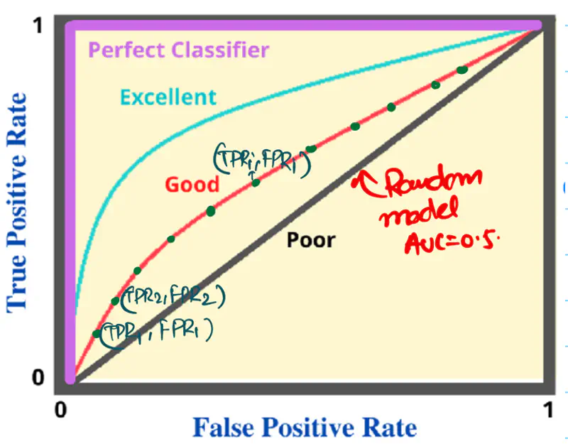
AU ROC = AUC = Area under the ROC curve = Area under the curve
Note:
- If AUC < 0.5, then invert the labels of the classes.
- ROC does NOT perform well on imbalanced data.
- Either balance the data or
- Use Precision-Recall curve.
Since, labels are randomly generated as 0/1 for binary classification, so 50% labels from each class.
Because random number generators generate numbers uniformly in the given range.
Let’s understand this with the below fraud detection example.
Below is a dataset from a fraud detection system for N = 10,000 transactions.
Fraud = 100, NOT fraud = 9900
| Predicted Fraud | Predicted NOT Fraud | |
|---|---|---|
| Actual Fraud | 80 (TP) | 20 (FN) |
| Actual NOT Fraud | 220 (FP) | 9680 (TN) |
If we check the location of above (TPR, FPR) pair on the ROC curve, then we can see that it is
very close to the top-left corner.
This means that the model is very good at detecting fraudulent transactions, but that is NOT the case.
This is happening because of the imbalanced data, i.e, count of NOT fraud transactions is 99 times
of fraudulent transactions.
Let’s look at the Precision value:
We can see that the model has poor precision,i.e, only 26.7% of flagged transactions are actual frauds.
Unacceptable precision for a good fraud detection system.
It is used to evaluate the performance of a binary classifier model across various thresholds.
It is similar to the ROC curve, but it uses Precision instead of TPR on the Y-axis.
Plots Precision (Y-axis) against Recall (X-axis) for different classification thresholds.
Note: It is useful when the data is imbalanced.
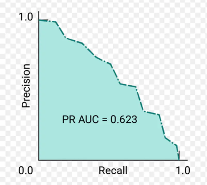
AU PRC = PR AUC = Area under Precision-Recall curve
Let’s revisit the fraud detection example discussed above to understand the utility of PR curve.
| Predicted Fraud | Predicted NOT Fraud | |
|---|---|---|
| Actual Fraud | 80 (TP) | 20 (FN) |
| Actual NOT Fraud | 220 (FP) | 9680 (TN) |
If we check the location of above (Precision, Recall) point on PRC curve, we will find that it is located near the
bottom right corner, i.e, the model performance is poor.
End of Section
3.1 - Vector Fundamentals
It is used to describe the surrounding space, e.g, lines, planes, 3D space, etc.
And, In machine learning, vectors are used to represent data, both the input features and the output of a model.
It is a collection of scalars(numbers) that has both magnitude and direction.
Geometrically, it is a line segment in space characterized by its length(magnitude) and direction.
By convention, we represent vectors as column vectors.
e.g.:
\(\vec{x} = \mathbf{x} = \begin{bmatrix} x_1 \\ x_2 \\ \vdots \\ x_n \end{bmatrix}_{\text{n×1}}\) i.e ’n’ rows and 1 column.
Important: In machine learning, we will use bold notation \(\mathbf{v}\) to represent vectors, instead
of arrow notation \(\mathbf{v}\).
Swap the rows and columns, i.e, a column vector becomes a row vector after transpose.
e.g:
\(\mathbf{v} = \begin{bmatrix} v_1 \\ v_2 \\ \vdots \\ v_d \end{bmatrix}_{\text{d×1}}\)
\(\mathbf{v}^\mathrm{T} = \begin{bmatrix} v_1 & v_2 & \cdots & v_d \end{bmatrix}_{\text{1×d}}\)
The length (or magnitude or norm) of a vector \(\mathbf{v}\) is the distance from the origin to the point represented
by \(\mathbf{v}\) in n-dimensional space.
\(\mathbf{v} = \begin{bmatrix} v_1 \\ v_2 \\ \vdots \\ v_d \end{bmatrix}_{\text{d×1}}\)
Length of vector:
Note: The length of a zero vector is 0.
The direction of a vector tells us where the vector points in space, independent of its length.
Direction of vector:
\[\mathbf{v} = \frac{\vec{v}} {\|\mathbf{v}\|} \]It is a collection of vectors that can be added together and scaled by numbers (scalars), such that,
the results are still in the same space.
Vector space or linear space is a non-empty set of vectors equipped with 2 operations:
- Vector addition: for any 2 vectors \(a, b\), \(a + b\) is also in the same vector space.
- Scalar multiplication: for a vector \(\mathbf{v}\), \(\alpha\mathbf{v}\) is also in the same vector space;
where \(\alpha\) is a scalar.
Note: These operations must satisfy certain rules (called axioms), such as, associativity, commutativity, distributivity, existence of a zero vector, and additive inverses.
e.g.: Set of all points in 2D is a vector space.
Addition:
We can only add vectors of the same dimension.
- Commutative: \(a + b = b + a\)
- Associative: \(a + (b + c) = (a + b) + c\)
e.g: lets add 2 real d-dimensional vectors, \(\mathbf{u} , \mathbf{v} \in \mathbb{R}^{d \times 1}\):
\(\mathbf{u} = \begin{bmatrix} u_1 \\ u_2 \\ \vdots \\ u_d \end{bmatrix}_{\text{d×1}}\),
\(\mathbf{v} = \begin{bmatrix} v_1 \\ v_2 \\ \vdots \\ v_d \end{bmatrix}_{\text{d×1}}\)
\(\mathbf{u} + \mathbf{v} = \begin{bmatrix} u_1+v_1 \\ u_2+v_2 \\ \vdots \\ u_d+v_d \end{bmatrix}_{\text{d×1}}\)
Multiplication:
1. Multiplication with Scalar:
All elements of the vector are multiplied with the scalar.
- \(c(\mathbf{u} + \mathbf{v}) = c(\mathbf{u}) + c(\mathbf{v})\)
- \((c+d)\mathbf{v} = c\mathbf{v} + d\mathbf{v}\)
- \((cd)\mathbf{v} = c(d\mathbf{v})\)
e.g:
\(\alpha\mathbf{v} = \begin{bmatrix} \alpha v_1 \\ \alpha v_2 \\ \vdots \\ \alpha v_d \end{bmatrix}_{\text{d×1}}\)
2.Inner (Dot) Product:
Inner(dot) product \(\mathbf{u} \cdot \mathbf{v}\) of 2 vectors gives a scalar output.
The two vectors must be of the same dimensions.
- \(\mathbf{u} \cdot \mathbf{v} = u_1v_1 + u_2v_2 + \cdots + u_dv_d\)
Dot product:
\(\mathbf{u} \cdot \mathbf{v} = \mathbf{u}^\mathrm{T} \mathbf{v}\)
= \(\begin{bmatrix} u_1 & u_2 & \cdots & u_d \end{bmatrix}_{\text{1×d}}
\cdot
\begin{bmatrix} v_1 \\ v_2 \\ \vdots \\ v_d
\end{bmatrix}_{\text{d×1}} = u_1v_1 + u_2v_2 + \cdots + u_dv_d\)
Geometrically, \(\mathbf{u} \cdot \mathbf{v}\) = \(|u||v|cos\theta\)
where \(\theta\) is the angle between \(\mathbf{u}\) and \(\mathbf{v}\).
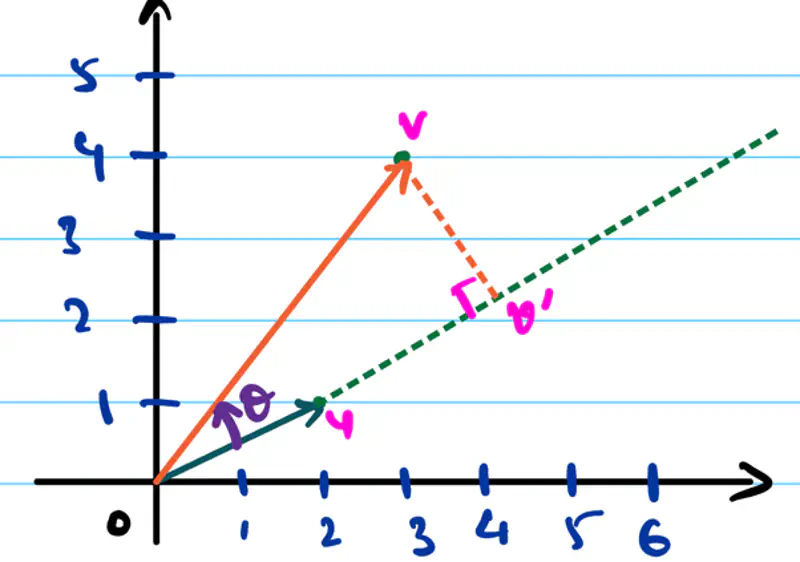
\(\mathbf{u} = \begin{bmatrix} 1 \\ \\ 2 \\ \end{bmatrix}_{\text{2×1}}\), \(\mathbf{v} = \begin{bmatrix} 3 \\ \\ 4 \\ \end{bmatrix}_{\text{2×1}}\)
\(\mathbf{u} \cdot \mathbf{v}\) = \(|u||v|cos\theta = 1 \times 3 + 2 \times 4 = 11\)
2.Outer (Tensor) Product:
Outer (tensor) product \(\mathbf{u} \otimes \mathbf{v}\) of 2 vectors gives a matrix output.
The two vectors must be of the same dimensions.
Tensor product:
\(\mathbf{u} \otimes \mathbf{v} = \mathbf{u} \mathbf{v}^\mathrm{T} \)
= \(\begin{bmatrix} u_1 \\ u_2 \\ \vdots \\ u_d \end{bmatrix}_{\text{d×1}}
\otimes
\begin{bmatrix} v_1 & v_2 & \cdots & v_d \end{bmatrix}_{\text{1×d}}
= \begin{bmatrix}
u_1v_1 & u_1v_2 & \cdots & u_1v_d \\
u_2v_1 & u_2v_2 & \cdots & u_2v_n \\
\vdots & \vdots & \ddots & \vdots \\
u_dv_1 & u_dv_2 & \cdots & u_dv_d
\end{bmatrix}
\in \mathbb{R}^{d \times d}\)
e.g:
\(\mathbf{u} = \begin{bmatrix} 1 \\ \\ 2 \\ \end{bmatrix}_{\text{2×1}}\),
\(\mathbf{v} = \begin{bmatrix} 3 \\ \\ 4 \\ \end{bmatrix}_{\text{2×1}}\)
\(\mathbf{u} \otimes \mathbf{v} = \mathbf{u} \mathbf{v}^\mathrm{T} \) = \(\begin{bmatrix} 1 \\ \\ 2 \\ \end{bmatrix}_{\text{2×1}} \otimes \begin{bmatrix} 3 & 4 \end{bmatrix}_{\text{1×2}} = \begin{bmatrix} 1 \times 3 & 1 \times 4 \\ \\ 2 \times 3 & 2 \times 4 \\ \end{bmatrix} _{\text{2×2}} = \begin{bmatrix} 3 & 4 \\ \\ 6 & 8 \\ \end{bmatrix} _{\text{2×2}}\)
Note: We will NOT discuss about cross product \(\mathbf{u} \times \mathbf{v}\); product perpendicular to both vectors.
\(\mathbf{v} = \alpha_1 \mathbf{u}_1 + \alpha_2 \mathbf{u}_2 + \cdots + \alpha_k \mathbf{u}_k\)
where \(\alpha_1, \alpha_2, \cdots, \alpha_k\) are scalars.
A set of vectors are linearly independent if NO vector in the set can be expressed as a linear combination of
the other vectors in the set.
The only solution for :
\(\alpha_1 \mathbf{u}_1 + \alpha_2 \mathbf{u}_2 + \cdots + \alpha_k \mathbf{u}_k\) = 0
is \(\alpha_1 = \alpha_2, \cdots, = \alpha_k = 0\).
e.g.:
The below 3 vectors are linearly independent.
\(\mathbf{u} = \begin{bmatrix} 1 \\ 1 \\ 1 \\ \end{bmatrix}_{\text{3×1}}\), \(\mathbf{v} = \begin{bmatrix} 1 \\ 2 \\ 3 \\ \end{bmatrix}_{\text{3×1}}\), \(\mathbf{w} = \begin{bmatrix} 1 \\ 3 \\ 6 \\ \end{bmatrix}_{\text{3×1}}\)The below 3 vectors are linearly dependent.
\(\mathbf{u} = \begin{bmatrix} 1 \\ 1 \\ 1 \\ \end{bmatrix}_{\text{3×1}}\), \(\mathbf{v} = \begin{bmatrix} 1 \\ 2 \\ 3 \\ \end{bmatrix}_{\text{3×1}}\), \(\mathbf{w} = \begin{bmatrix} 2 \\ 4 \\ 6 \\ \end{bmatrix}_{\text{3×1}}\)
because, \(\mathbf{w} = 2\mathbf{v}\), and we have a non-zero solution for the below equation:
\(\alpha_1 \mathbf{u} + \alpha_2 \mathbf{v} + \alpha_3 \mathbf{w} = 0\);
\(\alpha_1 = 0, \alpha_2 = -2, \alpha_3 = 1\) is a valid non-zero solution.
Note:
- A common method to check linear independence is to arrange the column vectors in a matrix form and calculate its determinant, if determinant ≠ 0, then the vectors are linearly independent.
- If number of vectors > number of dimensions, then the vectors are linearly dependent.
Since, the \((n+1)^{th}\) vector can be expressed as a linear combination of the other ’n’ vectors in n-dimensional space. - In machine learning, if a feature can be expressed in terms of other features, then it is linearly dependent,
and the feature is NOT bringing any new information.
e.g.: In 2 dimensions, 3 vectors \(\mathbf{x_1}, \mathbf{x_2}, \mathbf{x_3} \) are linearly dependent.
Span of a set of vectors is the geometric shape by all possible linear combinations of those vectors, such as,
line, plane, or higher dimensional volume.
e.g.:
- Span of a single vector (1,0) is the entire X-axis.
- Span of 2 vectors (1,0) and (0,1) is the entire X-Y (2D) plane, as any vector in 2D plane can be expressed as a linear combination of the 2 vectors - (1,0) and (0,1).
It is the minimal set of linearly independent vectors that spans or defines the entire vector space,
providing a unique co-ordinate system for every vector within the space.
Every vector in the vector space can be represented as a unique linear combination of the basis vectors.
e.g.:
- X-axis(1,0) and Y-axis(0,1) are the basis vectors of 2D space or form the co-ordinate system.
- \(\mathbf{u} = (3,1)\) and \(\mathbf{v} = (-1, 2) \) are the basis of skewed or parallelogram co-ordinate system.
Note: Basis = Dimensions
Two vectors are orthogonal if their dot product is 0.
A set of vectors \(\mathbf{x_1}, \mathbf{x_2}, \cdots ,\mathbf{x_n} \) are said to be orthogonal if:
\(\mathbf{x_i} \cdot \mathbf{x_j} = 0 \forall i⍯j\), for every pair, i.e, every pair must be orthogonal.
e.g.:
- \(\mathbf{u} = (1,0)\) and \(\mathbf{v} = (0,1) \) are orthogonal vectors.
- \(\mathbf{u} = (1,0)\) and \(\mathbf{v} = (1,1) \) are NOT orthogonal vectors.
Note:
Orthogonal vectors are linearly independent, but the inverse may NOT be true,
i.e, linear independence does NOT imply that vectors are orthogonal. e.g.:
Vectors \(\mathbf{u} = (2,0)\) and \(\mathbf{v} = (1,3) \) are linearly independent but NOT orthogonal.
Since, \(\mathbf{u} \cdot \mathbf{v} = 2*1 + 3*0 = 2 ⍯ 0\).Orthogonality is the most extreme case of linear independence, i.e \(90^{\degree}\) apart or perpendicular.
Orthonormal vectors are vectors that are orthogonal and have unit length.
A set of vectors \(\mathbf{x_1}, \mathbf{x_2}, \cdots ,\mathbf{x_n} \) are said to be orthonormal if:
\(\mathbf{x_i} \cdot \mathbf{x_j} = 0 \forall i⍯j\) and \(\|\mathbf{x_i}\| = 1\), i.e, unit vector.
e.g.:
- \(\mathbf{u} = (1,0)\) and \(\mathbf{v} = (0,1) \) are orthonormal vectors.
- \(\mathbf{u} = (1,0)\) and \(\mathbf{v} = (0,2) \) are NOT orthonormal vectors.
It is a set of vectors that functions as a basis for a space while also being orthonormal,
meaning each vector is a unit vector (has a length of 1) and all vectors are mutually perpendicular (orthogonal) to each other.
A set of vectors \(\mathbf{x_1}, \mathbf{x_2}, \cdots ,\mathbf{x_n} \) are said to be orthonormal basis of a vector space
\(\mathbb{R}^{n \times 1}\), if every vector:
e.g.:
- \(\mathbf{u} = (1,0)\) and \(\mathbf{v} = (0,1) \) form an orthonormal basis for 2-D space.
- \(\mathbf{u} = (\frac{1}{\sqrt{2}},\frac{1}{\sqrt{2}})\) and \(\mathbf{v} = (-\frac{1}{\sqrt{2}},-\frac{1}{\sqrt{2}}) \)
also form an orthonormal basis for 2-D space.
Note: In a n-dimensional space, there are only \(n\) possible orthonormal bases.
End of Section
3.2 - Matrix Operations
Matrices let us store, manipulate, and transform data efficiently.
e.g:
- Represent a system of linear equations AX=B.
- Data representation, such as images, that are stored as a matrix of pixels.
- When multiplied, matrix, linearly transforms a vector, i.e, its direction and magnitude, making it useful in image rotation, scaling, etc.
e.g:
\( \mathbf{A} = \begin{bmatrix} a_{11} & a_{12} & \cdots & a_{1n} \\ a_{21} & a_{22} & \cdots & a_{2n} \\ \vdots & \vdots & \ddots & \vdots \\ a_{m1} & a_{m2} & \cdots & a_{mn} \end{bmatrix} _{\text{m x n}} \)
\( \mathbf{A}^T = \begin{bmatrix} a_{11} & a_{21} & \cdots & a_{m1} \\ a_{12} & a_{22} & \cdots & a_{m2} \\ \vdots & \vdots & \ddots & \vdots \\ a_{1n} & a_{2n} & \cdots & a_{mn} \end{bmatrix} _{\text{n x m}} \)
Important: \( (AB)^T = B^TA^T \)
Addition:
We add two matrices by adding the corresponding elements.
They must have same dimensions.
\( \mathbf{A} + \mathbf{B} =
\begin{bmatrix}
a_{11} + b_{11} & a_{12} + b_{12} & \cdots & a_{1n} + b_{1n} \\
a_{21} + b_{21} & a_{22} + b_{22} & \cdots & a_{2n} + b_{2n} \\
\vdots & \vdots & \ddots & \vdots \\
a_{m1} + b_{m1} & a_{m2} + b_{m2} & \cdots & a_{mn} + b_{mn}
\end{bmatrix}
_{\text{m x n}}
\)
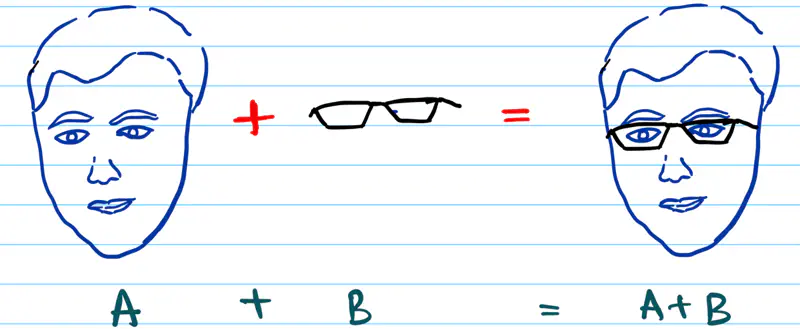
Multiplication:
We can multiply two matrices only if their inner dimensions are equal.
\( \mathbf{C}_{m x n} = \mathbf{A}_{m x d} ~ \mathbf{B}_{d x n} \)
\( c_{ij} \) = Dot product of \(i^{th}\) row of A and \(j^{th}\) row of B.
\( c_{ij} = \sum_{k=1}^{d} A_{ik} * B_{kj} \)
=> \( c_{11} = a_{11} * b_{11} + a_{12} * b_{21} + \cdots + a_{1d} * b_{d1} \)
e.g:
\(
\mathbf{A} =
\begin{bmatrix}
1 & 2 \\
\\
3 & 4
\end{bmatrix}
_{\text{2 x 2}},
\mathbf{B} =
\begin{bmatrix}
5 & 6 \\
\\
7 & 8
\end{bmatrix}
_{\text{2 x 2}}
\)
\(
\mathbf{C} = \mathbf{A} \times \mathbf{B} =
\begin{bmatrix}
1 * 5 + 2 * 7 & 1 * 6 + 2 * 8 \\
\\
3 * 5 + 4 * 7 & 3 * 6 + 4 * 8
\end{bmatrix}
_{\text{2 x 2}}
= \begin{bmatrix}
19 & 22 \\
\\
43 & 50
\end{bmatrix}
_{\text{2 x 2}}
\)
Key Properties:
- AB ≠ BA ; NOT commutative
- (AB)C = A(BC) ; Associative
- A(B+C) = AB+AC ; Distributive
Square Matrix:
It is a matrix with same number of rows and columns (m=n).
\(
\mathbf{A} =
\begin{bmatrix}
a_{11} & a_{12} & \cdots & a_{1n} \\
a_{21} & a_{22} & \cdots & a_{2n} \\
\vdots & \vdots & \ddots & \vdots \\
a_{n1} & a_{n2} & \cdots & a_{nn}
\end{bmatrix}
_{\text{n x n}}
\)
Diagonal Matrix:
It is a square matrix with all non-diagonal elements equal to zero.
e.g.:
\( \mathbf{D} =
\begin{bmatrix}
d_{11} & 0 & \cdots & 0 \\
0 & d_{22} & \cdots & 0 \\
\vdots & \vdots & \ddots & \vdots \\
0 & 0 & \cdots & d_{nn}
\end{bmatrix}
_{\text{n x n}}
\)
Note: Product of 2 diagonal matrices is a diagonal matrix.
Lower Triangular Matrix:
It is a square matrix with all elements above the diagonal equal to zero.
e.g.:
\( \mathbf{L} =
\begin{bmatrix}
l_{11} & 0 & \cdots & 0 \\
l_{21} & l_{22} & \cdots & 0 \\
\vdots & \vdots & \ddots & \vdots \\
l_{n1} & l_{n2} & \cdots & l_{nn}
\end{bmatrix}
_{\text{n x n}}
\)
Note: Product of 2 lower triangular matrices is an lower triangular matrix.
Upper Triangular Matrix:
It is a square matrix with all elements below the diagonal equal to zero.
e.g.:
\( \mathbf{U} =
\begin{bmatrix}
u_{11} & u_{12} & \cdots & u_{1n} \\
0 & u_{22} & \cdots & u_{2n} \\
\vdots & \vdots & \ddots & \vdots \\
0 & 0 & \cdots & u_{nn}
\end{bmatrix}
_{\text{n x n}}
\)
Note: Product of 2 upper triangular matrices is an upper triangular matrix.
Symmetric Matrix:
It is a square matrix that is equal to its own transpose, i.e, flip the matrix along its diagonal,
it remains unchanged.
\( \mathbf{A} = \mathbf{A}^T \)
e.g.:
\( \mathbf{S} =
\begin{bmatrix}
s_{11} & s_{12} & \cdots & s_{1n} \\
s_{12} & s_{22} & \cdots & s_{2n} \\
\vdots & \vdots & \ddots & \vdots \\
s_{1n} & s_{2n} & \cdots & s_{nn}
\end{bmatrix}
_{\text{n x n}}
\)
Note: Diagonal matrix is a symmetric matrix.
Skew Symmetric Matrix:
It is a square symmetric matrix where the elements across the diagonal have opposite signs.
Also called Anti Symmetric Matrix.
\( \mathbf{A} = -\mathbf{A}^T \)
e.g.:
\( \mathbf{S} =
\begin{bmatrix}
0 & s_{12} & \cdots & s_{1n} \\
-s_{12} & 0 & \cdots & s_{2n} \\
\vdots & \vdots & \ddots & \vdots \\
-s_{1n} & -s_{2n} & \cdots & 0
\end{bmatrix}
_{\text{n x n}}
\)
Note: Diagonal elements of a skew symmetric matrix are zero, since the number should be equal to its negative.
Identity Matrix:
It is a square matrix with all the diagonal values equal to 1, rest of the elements are equal to zero.
e.g.:
\( \mathbf{I} =
\begin{bmatrix}
1 & 0 & \cdots & 0 \\
0 & 1 & \cdots & 0 \\
\vdots & \vdots & \ddots & \vdots \\
0 & 0 & \cdots & 1
\end{bmatrix}
_{\text{n x n}}
\)
Important:
\( \mathbf{I} \times \mathbf{A} = \mathbf{A} \times \mathbf{I} = \mathbf{A} \)
Trace:
It is the sum of the elements on the main diagonal of a square matrix.
Note: Main diagonal is NOT defined for a rectangular matrix.
\( \text{trace}(A) = \sum_{i=1}^{n} a_{ii} = a_{11} + a_{22} + \cdots + a_{nn}\)
If \( \mathbf{A} \in \mathbb{R}^{m \times n} \), and \( \mathbf{B} \in \mathbb{R}^{n \times m} \), then
\( \text{trace}(AB)_{m \times m} = \text{trace}(BA)_{n \times n} \)
Determinant:
It is a scalar value that reveals crucial properties about the matrix and its linear transformation.
- If determinant = 0 => singular matrix, i.e linearly dependent rows or columns.
- Determinant is also equal to the scaling factor of the linear transformation.
\(a_{1j} \) = element in the first row and j-th column
\(M_{1j} \) = submatrix of the matrix excluding the first row and j-th column
If n = 2, then,
\( |A| = a_{11} \, a_{22} - a_{12} \, a_{21} \)
Singular Matrix:
A square matrix with linearly dependent rows or columns, i.e, determinant = 0.
A singular matrix collapses space, say, a 3D space, into a 2D space or a higher dimensional space
to a lower dimensional space, making the transformation impossible to reverse.
Hence, a singular matrix is NOT invertible; i.e, inverse does NOT exist.
Singular matrix is also NOT invertible, because the inverse has division by determinant, and its determinant is zero.
Also called rank deficient matrix, because the rank < number of dimensions of the matrix,
due to the presence of linearly dependent rows or columns.
e.g: Below is a linearly dependent 2x2 matrix.
\( \mathbf{A} =
\begin{bmatrix}
a_{11} & a_{12} \\
\\
\beta a_{11} & \beta a_{12}
\end{bmatrix}
_{\text{2 x 2}},
det(\mathbf{A}) =
a_{11}\cdot \beta a_{12} - a_{12} \cdot \beta a_{11} = 0
\)
Note:
- \( det(A) = det(A^T) \)
- \( det(\beta A) = \beta^n det(A) \), where n is the number of dimensions of A and \(\beta\) is a scalar.
Inverse:
It is a square matrix that when multiplied by the original matrix, gives the identity matrix.
\( \mathbf{A} \mathbf{A}^{-1} = \mathbf{A}^{-1} \mathbf{A} = \mathbf{I} \)
Steps to compute inverse of a matrix:
- Calculate the determinant of the matrix. \( |A| = \det(A) \)
- For each element \(a_{ij}\), compute its minor \(M_{ij}\).
\(M_{ij}\) is the determinant of the submatrix of the matrix excluding the i-th row and j-th column. - Form the co-factor matrix \(C_{ij}\), using the minor.
\( C_{ij} = (-1)^{\,i+j}\,M_{ij} \) - Take the transpose of the cofactor matrix to get the adjugate matrix.
\( \mathrm{adj}(A) = \mathrm{C}^\mathrm{T} \) - Compute the inverse:
\( A^{-1} = \frac{1}{|A|}\,\mathrm{adj}(A) = \frac{1}{|A|}\,\mathrm{C}^\mathrm{T}\)
e.g:
\(
\mathbf{A} =
\begin{bmatrix}
1 & 0 & 3\\
2 & 1 & 1\\
1 & 1 & 1 \\
\end{bmatrix}
_{\text{3 x 3}}
\),
Co-factor matrix:
\(
\mathbf{C} =
\begin{bmatrix}
0 & -1 & 1\\
3 & -2 & -1\\
-3 & 5 & 1 \\
\end{bmatrix}
_{\text{3 x 3}}
\)
Adjugate matrix, adj(A) =
\(
\mathbf{C}^\mathrm{T} =
\begin{bmatrix}
0 & 3 & -3\\
-1 & -2 & 5\\
1 & -1 & 1 \\
\end{bmatrix}
_{\text{3 x 3}}
\)
determinant of \( \mathbf{A} \) =
\(
\begin{vmatrix}
1 & 0 & 3\\
2 & 1 & 1\\
1 & 1 & 1 \\
\end{vmatrix}
= 0 -\cancel 1 + \cancel 1 + \cancel3 - 2 -\cancel1 -\cancel 3 + 5 + \cancel1 = 3
\)
\(
\mathbf{A}^{-1} = \frac{1}{|A|}\,\mathrm{adj}(A)
= \frac{1}{3}\,
\begin{bmatrix}
0 & 3 & -3\\
-1 & -2 & 5\\
1 & -1 & 1 \\
\end{bmatrix}
_{\text{3 x 3}}
\)
=> \(
\mathbf{A}^{-1} =
\begin{bmatrix}
0 & 1 & -1\\
-1/3 & -2/3 & 5/3\\
1/3 & -1/3 & 1/3 \\
\end{bmatrix}
_{\text{3 x 3}}
\)
Note:
- Inverse of an Identity matrix is the Identity matrix itself.
- Inverse of \( \beta \mathbf{A} = \frac{1}{\beta}\mathbf{A}^{-1} \).
- \( (\mathbf{A}^\mathrm{T})^{-1} = (\mathbf{A}^{-1})^\mathrm{T} \).
- Inverse of a diagonal matrix is a diagonal matrix with reciprocal of the diagonal elements.
- Inverse of a upper triangular matrix is the upper triangular matrix.
- Inverse of a lower triangular matrix is the lower triangular matrix.
- Symmetric matrix, if invertible, then \((\mathbf{A}^{-1})^\mathrm{T} = \mathbf{A}^{-1}\), since, \(\mathbf{A} = \mathbf{A}^\mathrm{T}\)
It is a square matrix that whose rows and columns are orthonormal vectors, i.e, they are perpendicular to each other
and have a unit length.
\( \mathbf{A} \mathbf{A}^\mathrm{T} = \mathbf{A}^\mathrm{T} \mathbf{A} = \mathbf{A} \mathbf{A}^{-1} = \mathbf{I} \)
=> \( \mathbf{A}^\mathrm{T} = \mathbf{A}^{-1} \)
Note:
- Orthogonal matrix preserves the length and angles of vectors, acting as rotation or reflection in geometry.
- The determinant of an orthogonal matrix is always +1 or -1, because \( \mathbf{A} \mathbf{A}^\mathrm{T} = \mathbf{I} \)
Let’s check out why the rows and columns of an orthogonal matrix are orthonormal.
\( \mathbf{A} =
\begin{bmatrix}
a_{11} & a_{12} \\
\\
a_{21} & a_{22}
\end{bmatrix}
_{\text{2 x 2}}
\),
=> \( \mathbf{A}^\mathrm{T} =
\begin{bmatrix}
a_{11} & a_{21} \\
\\
a_{12} & a_{22}
\end{bmatrix}
_{\text{2 x 2}}
\)
Since, \( \mathbf{A} \mathbf{A}^\mathrm{T} = \mathbf{I} \)
\(
\begin{bmatrix}
a_{11} & a_{12} \\
\\
a_{21} & a_{22}
\end{bmatrix}
\begin{bmatrix}
a_{11} & a_{21} \\
\\
a_{12} & a_{22}
\end{bmatrix}
= \begin{bmatrix}
a_{11}^2 + a_{12}^2 & a_{11}a_{21} + a_{12}a_{22} \\
\\
a_{21}a_{11} + a_{21}a_{12} & a_{21}^2 + a_{22}^2
\end{bmatrix}
= \begin{bmatrix}
1 & 0 \\
\\
0 & 1
\end{bmatrix}
\)
Equating the terms, we get:
\( a_{11}^2 + a_{12}^2 = 1 \) => row 1 is a unit vector
\( a_{21}^2 + a_{22}^2 = 1 \) => row 2 is a unit vector
\( a_{11}a_{21} + a_{12}a_{22} = 0 \) => row 1 and row 2 are orthogonal to each other, since dot product = 0
\( a_{21}a_{11} + a_{21}a_{12} = 0 \) => row 1 and row 2 are orthogonal to each other, since dot product = 0
Therefore, the rows and columns of an orthogonal matrix are orthonormal.
Let, \(\mathbf{Q}\) is an orthogonal matrix, and \(\mathbf{v}\) is a vector.
Let’s calculate the length of \( \mathbf{Q} \mathbf{v} \)
Therefore, linear transformation of a vector by an orthogonal matrix does NOT change its length.
\( 2x + y = 5 \)
\( x + 2y = 4 \)
Lets solve the system of equations using matrix:
\(\begin{bmatrix}
2 & 1 \\
\\
1 & 2
\end{bmatrix}
\)
\(
\begin{bmatrix}
x \\
\\
y
\end{bmatrix}
= \begin{bmatrix}
5 \\
\\
4
\end{bmatrix}
\)
The above equation can be written as:
\(\mathbf{AX} = \mathbf{B} \)
=> \( \mathbf{X} = \mathbf{A}^{-1} \mathbf{B} \)
\( \mathbf{A} = \begin{bmatrix}
2 & 1 \\
\\
1 & 2
\end{bmatrix},
\mathbf{B} = \begin{bmatrix}
5 \\
\\
4
\end{bmatrix},
\mathbf{X} = \begin{bmatrix}
x \\
\\
y
\end{bmatrix}
\)
Lets compute the inverse of A matrix:
\( \mathbf{A}^{-1} = \frac{1}{3}\begin{bmatrix}
2 & -1 \\
\\
-1 & 2
\end{bmatrix}
\)
Since, \( \mathbf{X} = \mathbf{A}^{-1} \mathbf{B} \)
=> \( \mathbf{X} = \begin{bmatrix}
x \\
\\
y
\end{bmatrix}
= \frac{1}{3}\begin{bmatrix}
2 & -1 \\
\\
-1 & 2
\end{bmatrix}
\begin{bmatrix}
5 \\
\\
4
\end{bmatrix}
= \frac{1}{3}\begin{bmatrix}
6 \\
\\
3
\end{bmatrix}
= = \begin{bmatrix}
2 \\
\\
1
\end{bmatrix}
\)
Therefore, \( x = 2 \) and \( y = 1 \).
End of Section
3.3 - Eigen Value Decomposition
It tells us about the characteristic properties of a matrix.
Multiplying a vector by a matrix can change the direction or magnitude or both of the vector.
\( \mathbf{A} = \begin{bmatrix}
2 & 1 \\
\\
1 & 2
\end{bmatrix}
\),
\(\mathbf{u} = \begin{bmatrix} 0 \\ \\ 1 \\ \end{bmatrix}\),
\(\mathbf{v} = \begin{bmatrix} 1 \\ \\ 1 \\ \end{bmatrix}\)
\(\mathbf{Au} = \begin{bmatrix} 1 \\ \\ 2 \\ \end{bmatrix}\) , \(\quad\)
\(\mathbf{Av} = \begin{bmatrix} 3 \\ \\ 3 \\ \end{bmatrix}\)
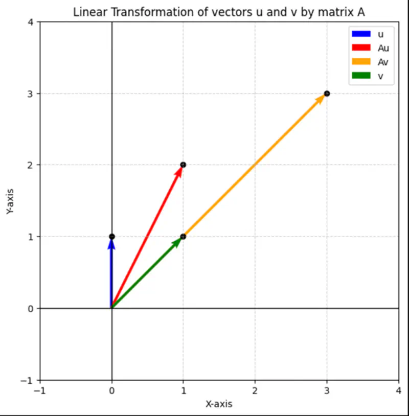
It might get scaled up or down but does not change its direction.
Result of linear transformation, i.e, multiplying the vector by a matrix, is just a scalar multiple of the original vector.
\(|\lambda| > 1 \): Vector stretched
\(0 < |\lambda| < 1 \): Vector shrunk
\(|\lambda| = 1 \): Same size
\(\lambda < 0 \): Vector’s direction is reversed
Since, for an eigen vector, result of linear transformation, i.e, multiplying the vector by a matrix, is just a scalar multiple of the original vector, =>
\[ \mathbf{A} \mathbf{v} = \lambda \mathbf{v} \\ \mathbf{A} \mathbf{v} - \lambda \mathbf{v} = 0 \\ \mathbf{v}(\mathbf{A} - \lambda \mathbf{I}) = 0 \\ \]For a non-zero eigen vector, \((\mathbf{A} - \lambda \mathbf{I})\) must be singular, i.e,
\(det(\mathbf{A} - \lambda \mathbf{I}) = 0 \)
If, \( \mathbf{A} =
\begin{bmatrix}
a_{11} & a_{12} & \cdots & a_{1n} \\
a_{21} & a_{22} & \cdots & a_{2n} \\
\vdots & \vdots & \ddots & \vdots \\
a_{n1} & a_{n2} & \cdots & a_{nn}
\end{bmatrix}
_{\text{n x n}}
\),
then, \((\mathbf{A} - \lambda \mathbf{I}) =
\begin{bmatrix}
a_{11}-\lambda & a_{12} & \cdots & a_{1n} \\
a_{21} & a_{22}-\lambda & \cdots & a_{2n} \\
\vdots & \vdots & \ddots & \vdots \\
a_{n1} & a_{n2} & \cdots & a_{nn}-\lambda
\end{bmatrix}
_{\text{n x n}}
\)
\(det(\mathbf{A} - \lambda \mathbf{I})) = 0 \), will give us a polynomial equation in \(\lambda\) of degree \(n\),
we need to solve this polynomial equation to get the \(n\) eigen values.
e.g.:
\( \mathbf{A} = \begin{bmatrix}
2 & 1 \\
\\
1 & 2
\end{bmatrix}
\),
\( \quad det(\mathbf{A} - \lambda \mathbf{I})) = 0 \quad \) =>
\( det \begin{bmatrix}
2-\lambda & 1 \\
\\
1 & 2-\lambda
\end{bmatrix} = 0
\)
\( (2-\lambda)^2 - 1 = 0\)
\( => |\lambda - 2| = \pm 1 \)
\( => \lambda_1 = 3\) and \( \lambda_2 = 1\)
Therefore, eigen vectors corresponding to eigen values \(\lambda_1 = 3\) and \( \lambda_2 = 1\) are:
\((\mathbf{A} - \lambda \mathbf{I}) \mathbf{v} = 0 \)
\(\lambda_1 = 3\)
=>
\(
\begin{bmatrix}
2-3 & 1 \\
\\
1 & 2-3
\end{bmatrix} \begin{bmatrix} v_1 \\ \\ v_2 \\ \end{bmatrix} =
\begin{bmatrix}
-1 & 1 \\
\\
1 & -1
\end{bmatrix} \begin{bmatrix} v_1 \\ \\ v_2 \\ \end{bmatrix} = 0
\)
=> Both the equations will be \(v_1 - v_2 = 0 \), i.e, \(v_1 = v_2\)
So, we can choose any vector, where x-axis and y-axis components are same, i.e, \(v_1 = v_2\)
=> Eigen vector: \(v_1 = \begin{bmatrix} 1 \\ \\ 1 \\ \end{bmatrix}\)
Similarly, for \(\lambda_2 = 1\)
we will get, eigen vector: \(v_2 = \begin{bmatrix} 1 \\ \\ -1 \\ \end{bmatrix}\)
\(\mathbf{Iv} = \lambda \mathbf{v}\)
Therefore, identity matrix has only one eigen value \(\lambda = 1\), and all non-zero vectors can be eigen vectors.
\(\mathbf{A} = \begin{bmatrix} 0 & 1 \\ \\ -1 & 0 \end{bmatrix} \), \( \quad det(\mathbf{A} - \lambda \mathbf{I}) = 0 \quad \) => det \(\begin{bmatrix} 0-\lambda & 1 \\ \\ -1 & 0-\lambda \end{bmatrix} = 0 \)
=> \(\lambda^2 + 1 = 0\) => \(\lambda = \pm i\)
So, eigen values are complex.
e.g.:
\( \mathbf{D} = \begin{bmatrix} d_{11} & 0 & \cdots & 0 \\ 0 & d_{22} & \cdots & 0 \\ \vdots & \vdots & \ddots & \vdots \\ 0 & 0 & \cdots & d_{nn} \end{bmatrix} _{\text{n x n}} \), \( \quad det(\mathbf{D} - \lambda \mathbf{I}) = 0 \quad \) => det \( \begin{bmatrix} d_{11}-\lambda & 0 & \cdots & 0 \\ 0 & d_{22}-\lambda & \cdots & 0 \\ \vdots & \vdots & \ddots & \vdots \\ 0 & 0 & \cdots & d_{nn}-\lambda \end{bmatrix} _{\text{n x n}} \)
=> \((d_{11}-\lambda)(d_{22}-\lambda) \cdots (d_{nn}-\lambda) = 0\)
=> \(\lambda = d_{11}, d_{22}, \cdots, d_{nn}\)
So, eigen values are the diagonal elements of the matrix.
- For a \(n \times n\) matrix, there are \(n\) eigen values.
- Eigen values need NOT be unique, e.g, identity matrix has only one eigen value \(\lambda = 1\).
- Sum of eigen values = trace of matrix = sum of diagonal elements, i.e,
\(tr(\mathbf{A}) = \lambda_1 + \lambda_2 + \cdots + \lambda_n\). - Product of eigen values = determinant of matrix, i.e,
\(det(\mathbf{A}) = |\mathbf{A}|= \lambda_1 \lambda_2 \cdots \lambda_n\). e.g: For the example matrix given above,
\( \mathbf{A} = \begin{bmatrix} 2 & 1 \\ \\ 1 & 2 \end{bmatrix} \), \(\quad \lambda_1 = 3\) and \( \lambda_2 = 1\)
\(tr(\mathbf{A}) = 2 + 2 = 3 + 1 = 4\)
\(det(\mathbf{A}) = 2 \times 2 - 1 \times 1 = 3 \times 1 = 3 \)
- Eigen vectors corresponding to distinct eigen values of a real symmetric matrix are orthogonal to each other.
Proof:
Let, \(\mathbf{v_1}, \mathbf{v_2}\) be eigen vectors corresponding to distinct eigen value \(\lambda_1,\lambda_2\) of a real symmetric matrix \(\mathbf{A} = \mathbf{A}^T\).
We know that for eigen vectors -
\[ \mathbf{Av_1} = \lambda_1 \mathbf{v_1} ~and~ \mathbf{Av_2} = \lambda_2 \mathbf{v_2} \\[10pt] \text{ let's calculate the dot product: } \\[10pt] \mathbf{Av_1} \cdot \mathbf{v_2} = (\mathbf{Av_1})^T\mathbf{v_2} = \mathbf{v_1^TA^Tv_2} = \mathbf{v_1^T} ~ \mathbf{Av_2}, \quad \text {since } \mathbf{A} = \mathbf{A}^T\\[10pt] => (\mathbf{Av_1}) \cdot \mathbf{v_2} = \mathbf{v_1} \cdot (\mathbf{Av_2}) \\[10pt] => (\lambda_1 \mathbf{v_1}) \cdot \mathbf{v_2} = \mathbf{v_1} \cdot (\lambda_2\mathbf{v_2}) \\[10pt] => \lambda_1 (\mathbf{v_1 \cdot v_2}) = \lambda_2 (\mathbf{v_1 \cdot v_2}) \\[10pt] => (\lambda_1 - \lambda_2) (\mathbf{v_1} \cdot \mathbf{v_2}) = 0 \\[10pt] \text{ since, eigen values are distinct,} => \lambda_1 ≠ \lambda_2 \\[10pt] \therefore \mathbf{v_1} \cdot \mathbf{v_2} = 0 \\[10pt] => \text{ eigen vectors are orthogonal to each other,} => \mathbf{v_1} \perp \mathbf{v_2} \\[10pt] \]
Let’ calculate the 2nd power of a square matrix.
e.g.:
\(\mathbf{A} = \begin{bmatrix}
2 & 1 \\
\\
1 & 2
\end{bmatrix}
\),
\(\quad \mathbf{A}^2 = \begin{bmatrix}
2 & 1 \\
\\
1 & 2
\end{bmatrix} \begin{bmatrix}
2 & 1 \\
\\
1 & 2
\end{bmatrix} = \begin{bmatrix}
5 & 4 \\
\\
4 & 5
\end{bmatrix}
\)
So, we need to find an easier way to calculate the power of a matrix.
Let’s calculate the 2nd power of a diagonal matrix.
e.g.:
\(\mathbf{A} = \begin{bmatrix}
3 & 0 \\
\\
0 & 2
\end{bmatrix}
\),
\(\quad \mathbf{A}^2 = \begin{bmatrix}
3 & 0 \\
\\
0 & 2
\end{bmatrix} \begin{bmatrix}
3 & 0 \\
\\
0 & 2
\end{bmatrix} = \begin{bmatrix}
9 & 0 \\
\\
0 & 4
\end{bmatrix}
\)
Note that when we square the diagonal matrix, then all the diagonal elements got squared.
Similarly, if we want to calculate the kth power of a diagonal matrix, then all we need to do is to just compute the kth
powers of all diagonal elements, instead of complex matrix multiplications.
\(\quad \mathbf{A}^k = \begin{bmatrix}
3^k & 0 \\
\\
0 & 2^k
\end{bmatrix}
\)
Therefore, if we diagonalize a square matrix then the computation of power of the matrix will become very easy.
Next, let’s see how to diagonalize a matrix.
\(\mathbf{V}\): Matrix of all eigen vectors(as columns) of matrix \(\mathbf{A}\)
\( \mathbf{V} = \begin{bmatrix}
\mathbf{v}_1 & \mathbf{v}_2 & \cdots & \mathbf{v}_n \\
\vdots & \vdots & \ddots & \vdots \\
\vdots & \vdots & \vdots & \vdots\\
\end{bmatrix}
\),
where, each column is an eigen vector corresponding to an eigen value \(\lambda_i\).
If \( \mathbf{v}_1 \mathbf{v}_2 \cdots \mathbf{v}_n \) are linearly independent, then,
\(det(\mathbf{V}) ~⍯ ~ 0\).
=> \(\mathbf{V}\) is NOT singular and \(\mathbf{V}^{-1}\) exists.
\(\Lambda\): Diagonal matrix of all eigen values of matrix \(\mathbf{A}\)
\( \Lambda = \begin{bmatrix}
\lambda_1 & 0 & \cdots & 0 \\
\\
0 & \lambda_2 & \cdots & 0 \\
\vdots & \vdots & \ddots & \vdots \\
0 & 0 & \cdots & \lambda_n
\end{bmatrix}
\),
where, each diagonal element is an eigen value corresponding to an eigen vector \(\mathbf{v}_i\).
Let’s recall the characteristic equation of a matrix for calculating eigen values:
\(\mathbf{A} \mathbf{v} = \lambda \mathbf{v}\)
Let’s use the consolidated matrix for eigen values and eigen vectors described above:
i.e, \(\mathbf{A} \mathbf{V} = \mathbf{\Lambda} \mathbf{V}\)
For diagonalisation:
=> \(\mathbf{\Lambda} = \mathbf{V}^{-1} \mathbf{A} \mathbf{V}\)
We can see that, using the above equation, we can represent the matrix \(\mathbf{A}\) as a
diagonal matrix \(\mathbf{\Lambda}\) using the matrix of eigen vectors \(\mathbf{V}\).
Just reshuffling the above equation will give us the Eigen Value Decomposition of the matrix \(\mathbf{A}\):
\(\mathbf{A} = \mathbf{V} \mathbf{\Lambda} \mathbf{V}^{-1}\)
Important: Given that \(\mathbf{V}^{-1}\) exists, i.e, all the eigen vectors are linearly independent.
Let’s revisit the example given above:
\(\mathbf{A} = \begin{bmatrix}
2 & 1 \\
\\
1 & 2
\end{bmatrix}
\),
\(\quad \lambda_1 = 3\) and \( \lambda_2 = 1\),
\(\mathbf{v_1} = \begin{bmatrix} 1 \\ \\ 1 \\ \end{bmatrix}\),
\(\mathbf{v_2} = \begin{bmatrix} 1 \\ \\ -1 \\ \end{bmatrix}\)
=> \( \mathbf{V} = \begin{bmatrix}
1 & 1 \\
\\
1 & -1 \\
\end{bmatrix}
\),
\(\quad \mathbf{\Lambda} = \begin{bmatrix}
3 & 0 \\
\\
0 & 1
\end{bmatrix}
\)
\( \because \mathbf{A} = \mathbf{V} \mathbf{\Lambda} \mathbf{V}^{-1}\)
We know, \( \mathbf{V} ~and~ \mathbf{\Lambda} \), we need to calculate \(\mathbf{V}^{-1}\).
\(\mathbf{V}^{-1} = \frac{1}{2}\begin{bmatrix} 1 & 1 \\ \\ 1 & -1 \\ \end{bmatrix} \)
\( \therefore \mathbf{V} \mathbf{\Lambda} \mathbf{V}^{-1} = \begin{bmatrix}
1 & 1 \\
\\
1 & -1 \\
\end{bmatrix} \begin{bmatrix}
3 & 0 \\
\\
0 & 1
\end{bmatrix} \frac{1}{2}\begin{bmatrix}
1 & 1 \\
\\
1 & -1 \\
\end{bmatrix}
\)
\( = \frac{1}{2}
\begin{bmatrix}
3 & 1 \\
\\
3 & -1 \\
\end{bmatrix} \begin{bmatrix}
1 & 1 \\
\\
1 & -1 \\
\end{bmatrix} = \frac{1}{2}\begin{bmatrix}
4 & 2 \\
\\
2 & 4 \\
\end{bmatrix}
\)
\( = \begin{bmatrix}
2 & 1 \\
\\
1 & 2
\end{bmatrix} = \mathbf{A}
\)
Spectral decomposition is a specific type of eigendecomposition that applies to a symmetric matrix,
requiring its eigenvectors to be orthogonal.
In contrast, a general eigendecomposition applies to any diagonalizable matrix and does not require the eigenvectors
to be orthogonal.
The eigen vectors corresponding to distinct eigen values are orthogonal.
However, the matrix \(\mathbf{V}\) formed by the eigen vectors as columns is NOT orthogonal,
because the rows/columns are NOT orthonormal i.e unit length.
So, in order to make the matrix \(\mathbf{V}\) orthogonal, we need to normalize the rows/columns of the matrix
\(\mathbf{V}\), i.e, make, each eigen vector(column) unit length, by dividing the vector by its magnitude.
After normalisation we get orthogonal matrix \(\mathbf{Q}\) that is composed of unit length and orthogonal eigen vectors
or orthonormal eigen vectors.
Since, matrix \(\mathbf{Q}\) is orthogonal, => \(\mathbf{Q}^T = \mathbf{Q}^{-1}\)
The eigen value decomposition of a square matrix is:
\(\mathbf{A} = \mathbf{V} \mathbf{\Lambda} \mathbf{V}^{-1}\)
And, the spectral decomposition of a real symmetric matrix is:
\(\mathbf{A} = \mathbf{Q} \mathbf{\Lambda} \mathbf{Q}^T\)
Important: Note that, we are discussing only the special case of real symmetric matrix here,
because a real symmetric matrix is guaranteed to have all real eigenvalues.
- Principal Component Analysis (PCA): For dimensionality reduction.
- Page Rank Algorithm: For finding the importance of a web page.
- Structural Engineering: By calculating the eigen values of a bridge’s structural model, we can identify its natural frequencies to ensure that the bridge won’t resonate and be damaged by external forces, such as wind, and seismic waves.
End of Section
3.4 - Singular Value Decomposition
It decomposes any matrix into a rotation, a scaling (based on singular values), and another rotation.
It is a generalization of the eigen value decomposition(for square matrix) to rectangular matrices.
Any rectangular matrix can be decomposed into a product of three matrices using SVD, as follows:
\(\mathbf{U}\): Set of orthonormal eigen vectors of \(\mathbf{AA^T}_{m \times m} \)
\(\mathbf{V}\): Set of orthonormal eigen vectors of \(\mathbf{A^TA}_{n \times n} \)
\(\mathbf{\Sigma}\): Rectangular diagonal matrix, whose diagonal values are called singular values;
square root of non-zero eigen values of \(\mathbf{AA^T}\).
Note: The number of non-zero diagonal entries in \(\mathbf{\Sigma}\) = rank of matrix \(\mathbf{A}\).
Rank (r): Number of linearly independent rows or columns of a matrix.
\( \Sigma = \begin{bmatrix}
\sigma_{11} & 0 & \cdots & 0 \\
\\
0 & \sigma_{22} & \cdots & 0 \\
\vdots & \vdots & \ddots & \vdots \\
\cdots & \cdots & \sigma_{rr} & \vdots \\
0 & 0 & \cdots & 0
\end{bmatrix}
\),
such that, \(\sigma_{11} \geq \sigma_{22} \geq \cdots \geq \sigma_{rr}\), r = rank of \(\mathbf{A}\).
Singular value decomposition, thus refers to the set of scale factors \(\mathbf{\Sigma}\) that are fundamentally
linked to the matrix’s singularity and rank.
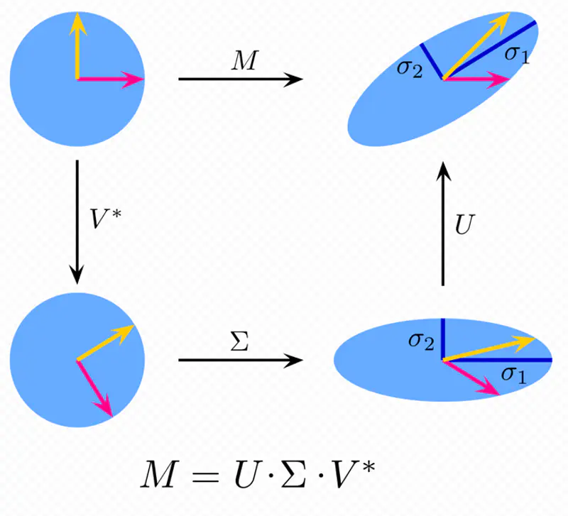
- All singular values are non-negative.
- Square roots of the eigen values of the matrix \(\mathbf{AA^T}\) or \(\mathbf{A^TA}\).
- Arranged in non-decreasing order.
\(\sigma_{11} \geq \sigma_{22} \geq \cdots \geq \sigma_{rr} \ge 0\)
Note: If rank of matrix < dimensions, then 1 or more of the singular values are zero, i.e, dimension collapse.
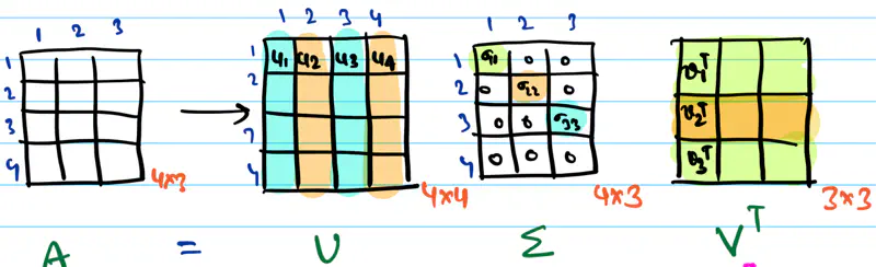
How can we compress the image size to save satellite bandwidth?
We can perform singular value decomposition on the image matrix and find the minimum number of top ranks required to
to successfully reconstruct the original image back.
Say we performed the SVD on the image matrix and found that top 20 rank singular values, out of 1000, are sufficient to
tell what the picture is about.
\(\mathbf{A} = \mathbf{U} \mathbf{\Sigma} \mathbf{V}^T \)
\( = u_1 \sigma_1 v_1^T + u_2 \sigma_2 v_2^T + \cdots + u_r \sigma_r v_r^T \), where \(r = 20\)
A = sum of ‘r=20’ matrices of rank=1.
Now, we need to send only the \(u_i, \sigma_i , v_i\) values for i=20, i.e, top 20 ranks to earth
and then do the calculation to reconstruct the approximation of original image.
\(\mathbf{u} = \begin{bmatrix} u_1 \\ u_2 \\ \vdots \\ u_{1000} \end{bmatrix}\)
\(\mathbf{v} = \begin{bmatrix} v_1 \\ v_2 \\ \vdots \\ v_{1000} \end{bmatrix}\)
So, we need to send data corresponding to 20 (rank=1) matrices, i.e, \(u_i, v_i ~and~ \sigma_i\) = (1000 + 1000 + 1)20 = 200020 pixels (approx)
Therefore, compression rate = (2000*20)/(10^6) = 1/25
- Image compression.
- Low Rank Approximation: Compress data by keeping top rank singular values.
- Noise Reduction: Capture main structure, ignore small singular values.
- Recommendation Systems: Decompose user-item rating matrix to discover underlying user preferences and make recommendations.
The process of approximating any matrix by a matrix of a lower rank, using singular value decomposition.
It is used for data compression.
Any matrix A of rank ‘r’ can be written as sum of rank=1 outer products:
\[ \mathbf{A} = \mathbf{U} \mathbf{\Sigma} \mathbf{V}^T = \sum_{i=1}^{r} \sigma_i \mathbf{u}_i \mathbf{v}_i^T \]\( \mathbf{u}_i : i^{th}\) column vector of \(\mathbf{U}\)
\( \mathbf{v}_i^T : i^{th}\) column vector of \(\mathbf{V}^T\)
\( \sigma_i : i^{th}\) singular value, i.e, diagonal entry of \(\mathbf{\Sigma}\)
Since, the singular values are arranged from largest to smallest, i.e, \(\sigma_1 \geq \sigma_2 \geq \cdots \geq \sigma_r\),
The top ranks capture the vast majority of the information or variance in the matrix.
So, in order to get the best rank-k approximation of the matrix,
we simply truncate the summation after the k’th term.
The approximation \(\mathbf{A_k}\) is called the low rank approximation of \(\mathbf{A}\),
which is achieved by keeping only the largest singular values and corresponding vectors.
Applications:
- Image compression
- Data compression, such as, LoRA (Low Rank Adaptation)
End of Section
3.5 - Principal Component Analysis
In the diagram below, if we need to reduce the dimensionality of the data to 1, which feature should be dropped?
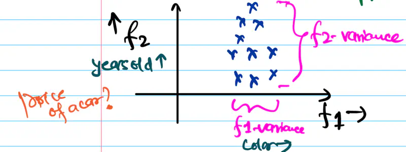
Since, information = variance, we should drop the feature that brings least information, i.e, has least variance.
Therefore, drop the feature 1.
What if the variance in both directions is same ?
What should be done in this case? Check the diagram below.
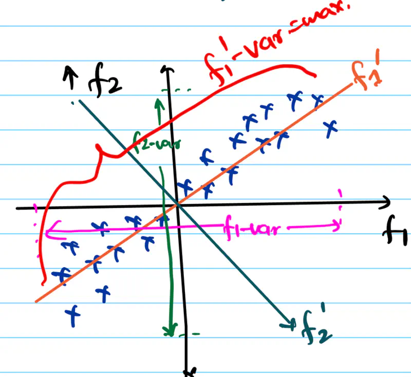
we will rotate the f1-axis in the direction of maximum spread/variance of data, i.e, f1’-axis and then we can drop f2’-axis, which is perpendicular to f1’-axis.
It is a dimensionality reduction technique that finds the direction of maximum variance in the data.
Note: Some loss of information will always be there in dimensionality reduction, because there will be some variability
in data along the direction that is dropped, and that will be lost.
Goal:
Fundamental goal of PCA is to find the new set of orthogonal axes, called the principal components, onto which
the data can be projected, such that, the variance of the projected data is maximum.
Note: Modern libraries (like sklearn.decomposition.PCA) default to Singular Value Decomposition (SVD) for PCA; but we will use Eigen Value Decomposition to understand the algorithm.
Say, we have data, \(D:X \in \mathbb{R}^{n \times d}\),
n is the number of samples
d is the number of features or dimensions of each data point.
In order to find the directions of maximum variance in data, we will use the covariance matrix of data.Covariance matrix (C) summarizes the spread and relationship of the data in the original d-dimensional space.
- \(C_{d \times d} = \frac{1}{n-1}X^TX \), where \(X\) is the data matrix.
- \(C_{d \times d} = \frac{1}{n-1}X^TX \), where \(X\) is the data matrix.
Note: (n-1) in the denominator is for unbiased estimation(Bessel’s correction) of covariance matrix.
- \(C_{ii}\) is the variance of the \(i^{th}\) feature.
- \(C_{ij}\) is the co-variance between feature \(i\) and feature \(j\).
- Trace(C) = Sum of diagonal elements of C = Total variance of data.
Algorithm:
- Data is first mean centered, i.e, make mean = 0, i.e, subtract mean from each data point.
- \(X = X - \mu\)
- Compute the covariance matrix with mean centered data.
- \(C = \frac{1}{n-1}X^TX \), \( \quad C ~ \text{or } \Sigma = \begin{bmatrix} var(f_1) & cov(f_1f_2) & \cdots & cov(f_1f_d) \\ cov(f_2f_1) & var(f_2) & \cdots & cov(f_2f_d) \\ \vdots & \vdots & \ddots & \vdots \\ cov(f_df_1) & cov(f_df_2) & \cdots & var(f_d) \end{bmatrix} _{\text{d x d}} \)
- Perform the eigen value decomposition of covariance matrix.
- \( C = Q \Lambda Q^T \)
- \(C\): Orthogonal matrix of eigen vectors of covariance matrix.
- New rotated axes or principal components of the data.
- New rotated axes or principal components of the data.
- \(\Lambda\): Diagonal matrix of eigen values of covariance matrix.
- Scaling of variance along new eigen basis.
- Scaling of variance along new eigen basis.
Note: Eigen values are sorted in descending order, i.e \( \lambda_1 \geq \lambda_2 \geq \cdots \geq \lambda_d \).
- Project the data onto the new axes or principal components/directions.
Note: k < d = reduced dimensionality.
\(X_{new} = Z = XQ_k\)
\(X_{new}\): Projected data or principal component score
Variance of projected data is given by the eigen value of the co-variance matrix.
Covariance of projected data = \((XQ)^TXQ \)
Therefore, the diagonal matrix \( \Lambda \) captures the variance along every principal component direction.
End of Section
3.6 - Vector & Matrix Calculus
Let \(\mathbf{x} = \begin{bmatrix} x_1 \\ x_2 \\ \vdots \\ x_n \end{bmatrix}_{\text{n×1}}\) be a vector, i.e, \(\mathbf{x} \in \mathbb{R}^n\).
Let \(f(x)\) be a function that maps a vector to a scalar, i.e, \(f : \mathbb{R}^n \rightarrow \mathbb{R}\).
The derivative of function \(f(x)\) with respect to \(\mathbf{x}\) is defined as:
Assumption: All the first order partial derivatives exist.
e.g.:
- \(f(x) = a^Tx\), where,
\(\mathbf{x} = \begin{bmatrix} x_1 \\ x_2 \\ \vdots \\ x_n \end{bmatrix}\),
\(\quad a = \begin{bmatrix} a_1 \\ a_2 \\ \vdots \\ a_n \end{bmatrix}\),
\(\quad a^T = \begin{bmatrix} a_1 & a_2 & \cdots & a_n \end{bmatrix}\)
\(=> f(x) = a^Tx = a_1x_1 + a_2x_2 + \cdots + a_nx_n\)
\(=> \frac{\partial f(x)}{\partial x} = \begin{bmatrix} \frac{\partial x_1}{\partial x} \\ \frac{\partial x_2}{\partial x} \\ \vdots \\ \frac{\partial x_n}{\partial x} \end{bmatrix} \) \(=\begin{bmatrix} a_1 \\ a_2 \\ \vdots \\ a_n \end{bmatrix} = a \)
\( => f'(x) = a \)
- Now, let’s find the derivative for a bit complex, but very widely used function.
\(f(x) = \mathbf{x^TAx} \quad\), where, \(\mathbf{x} = \begin{bmatrix} x_1 \\ x_2 \\ \vdots \\ x_n \end{bmatrix}\), so, \(\quad x^T = \begin{bmatrix} x_1 & x_2 & \cdots & x_n \end{bmatrix}\),
A is a square matrix, \( \mathbf{A} = \begin{bmatrix} a_{11} & a_{12} & \cdots & a_{1k} & \cdots a_{1n} \\ a_{21} & a_{22} & \cdots & a_{2k} & \cdots a_{2n} \\ \vdots & \vdots & \ddots & \vdots & \vdots \\ a_{k1} & a_{k2} & \cdots & a_{kk} & \cdots a_{kn} \\ \vdots & \vdots & \ddots & \vdots & \vdots \\ a_{n1} & a_{n2} & \cdots & a_{nk} & \cdots a_{nn} \end{bmatrix} _{\text{n x n}} \)
So, \( \mathbf{A^T} = \begin{bmatrix} a_{11} & a_{21} & \cdots & a_{k1} & \cdots a_{n1} \\ a_{12} & a_{22} & \cdots & a_{k2} & \cdots a_{n2} \\ \vdots & \vdots & \ddots & \vdots & \vdots \\ a_{1k} & a_{2k} & \cdots & a_{kk} & \cdots a_{nk} \\ \vdots & \vdots & \ddots & \vdots & \vdots \\ a_{1n} & a_{2n} & \cdots & a_{kn} & \cdots a_{nn} \end{bmatrix} _{\text{n x n}} \)
Let’s calculate \(\frac{\partial y}{\partial x_k}\), i.e, for the \(k^{th}\) element and sum it over 1 to n.
The \(k^{th}\) element \(x_k\) will appear 2 times in the below summation, i.e, when \(i=k ~and~ j=k\)
Above, we saw the gradient of a scalar valued function, i.e, a function that maps a vector to a scalar, i.e,
\(f : \mathbb{R}^n \rightarrow \mathbb{R}\).
There is another kind of function called vector valued function, i.e, a function that maps a vector to another vector, i.e,
\(f : \mathbb{R}^n \rightarrow \mathbb{R}^m\).
The Jacobian is the matrix of all first-order partial derivatives of a vector-valued function,
while the gradient is a vector representing the partial derivatives of a scalar-valued function.
- Jacobian matrix provides the best linear approximation of a vector valued function near a given point,
similar to how a derivative/gradient is the best linear approximation for a scalar valued function
Note: Gradient is a special case of the Jacobian;
it is the transpose of the Jacobian for a scalar valued function.
Let, \(f(x)\) be a function that maps a vector to another vector, i.e, \(f : \mathbb{R}^n \rightarrow \mathbb{R}^m\)
\(f(x)_{m \times 1} = \mathbf{A_{m \times n}x_{n \times 1}}\), where,
\(\quad
\mathbf{A} =
\begin{bmatrix}
a_{11} & a_{12} & \cdots & a_{1n} \\
a_{21} & a_{22} & \cdots & a_{2n} \\
\vdots & \vdots & \ddots & \vdots \\
a_{m1} & a_{m2} & \cdots & a_{mn}
\end{bmatrix}
_{\text{m x n}}
\),
\(\mathbf{x} = \begin{bmatrix} x_1 \\ x_2 \\ \vdots \\ x_n \end{bmatrix}_{\text{n x 1}}\),
\(f(x) = \begin{bmatrix} f_1(x) \\ f_2(x) \\ \vdots \\ f_m(x) \end{bmatrix}_{\text{m x 1}}\)
The above matrix is called Jacobian matrix of \(f(x)\).
Assumption: All the first order partial derivatives exist.
Hessian Matrix:
It is a square matrix of second-order partial derivatives of a scalar-valued function.
This is used to characterize the curvature of a function at a give point.
Let, \(f(x)\) be a function that maps a vector to a scalar value, i.e, \(f : \mathbb{R}^n \rightarrow \mathbb{R}\)
The Hessian matrix is defined as:
Note: Most functions in Machine Learning where second-order partial derivatives are continuous, the Hessian is symmetrix.
\( H_{i,j} = H_{j,i} = \frac{\partial f^2(x)}{\partial x_i \partial x_j } = \frac{\partial f^2(x)}{\partial x_j \partial x_i } \)
e.g:
\(f(x) = \mathbf{x^TAx}\), where, A is a symmetric matrix, and f(x) is a scalar valued function.
\(Gradient = \frac{\partial }{\partial x}(\mathbf{x^TAx}) = 2\mathbf{Ax}\), since A is symmetric.
\(Hessian = \frac{\partial^2 }{\partial x^2}(\mathbf{x^TAx}) = \frac{\partial }{\partial x}2\mathbf{Ax} = 2\mathbf{A}\)\(f(x,y) = x^2 + y^2\)
\(Gradient = \nabla f = \begin{bmatrix} \frac{\partial f}{\partial x}\\ \\ \frac{\partial f}{\partial x} \end{bmatrix} = \begin{bmatrix} 2x+0 \\ \\ 0+2y \end{bmatrix} = \begin{bmatrix} 2x \\ \\ 2y \end{bmatrix}\)
\(Hessian = \nabla^2 f = \begin{bmatrix} \frac{\partial^2 f}{\partial x^2} & \frac{\partial^2 f}{\partial x \partial y}\\ \\ \frac{\partial^2 f}{\partial y \partial x} & \frac{\partial^2 f}{\partial y^2} \end{bmatrix} = \begin{bmatrix} 2 & 0 \\ \\ 0 & 2 \end{bmatrix}\)
Let, A is a mxn matrix, i.e \(A \in \mathbb{R}^{m \times n}\)
\(\mathbf{A} =
\begin{bmatrix}
a_{11} & a_{12} & \cdots & a_{1n} \\
a_{21} & a_{22} & \cdots & a_{2n} \\
\vdots & \vdots & \ddots & \vdots \\
a_{m1} & a_{m2} & \cdots & a_{mn}
\end{bmatrix}
_{\text{m x n}}
\)
Let f(A) be a function that maps a matrix to a scalar value, i.e, \(f : \mathbb{R}^{m \times n} \rightarrow \mathbb{R}\)
, then derivative of function f(A) w.r.t A is defined as:
e.g.:
- Let, A is a square matrix, i.e \(A \in \mathbb{R}^{n \times n}\)
and f(A) = trace(A) = \(a_{11} + a_{22} + \cdots + a_{nn}\)
We know that:
\((\frac{\partial f}{\partial A})_{(i,j)} = \frac{\partial f}{\partial a_{ij}}\)
Since, the trace only contains diagonal elements,
=> \((\frac{\partial f}{\partial A})_{(i,j)}\) = 0 for all \(i ⍯ j\)
similarly, \((\frac{\partial f}{\partial A})_{(i,i)}\) = 1 for all \(i=j\)
=> \( \frac{\partial Tr(A)}{\partial A} = \begin{cases} 1, & \text{if } i=j \\ \\ 0, & \text{if } i⍯j \end{cases} \)
\(\frac{\partial f}{\partial A} = \frac{\partial Tr(A)}{\partial A} \begin{bmatrix} 1 & 0 & \cdots & 0 \\ 0 & 1& \cdots & 0 \\ \vdots & \vdots & \ddots & \vdots \\ 0 & 0 & \cdots & 1 \end{bmatrix} = \mathbf{I} \)
Therefore, derivative of trace(A) w.r.t A is an identity matrix.
End of Section
3.7 - Vector Norms
It is a measure of the size of a vector or distance from the origin.
Vector norm is a function that maps a vector to a real number, i.e, \({\| \cdot \|} : \mathbb{R}^n \rightarrow \mathbb{R}\).
Vector Norm should satisfy following 3 properties:
- Non-Negativity:
Norm is always greater than or equal to zero,
\( {\| x \|} \ge 0\), and \( {\| x \|} = 0\), if and only if \(\vec{x} = \vec{0}\). - Homogeneity (or Scaling):
\( {\| \alpha x \|} = |\alpha| {\| x \|} \). - Triangle Inequality:
\( {\| x + y \|} \le {\| x \|} + {\| y \|} \).
P-Norm:
It is a generalised form of most common family of vector norms, also called Minkowski norm.
It is defined as:
We can change the value of \(p\) to get different norms.
L1 Norm:
It is the sum of absolute values of all the elements of a vector; also known as Manhattan distance.
p=1:
L2 Norm:
It is the square root of the sum of squares of all the elements of a vector; also known as Euclidean distance.
p=2:
L-\(\infty\) Norm:
It is the maximum of absolute values of all the elements of a vector; also known as Chebyshev distance.
p=\(\infty\):
- Let, vector \(\mathbf{x} = \begin{bmatrix} 3 \\ \\ -4 \end{bmatrix}\), then
\({\| x \|_1} = |3| + |-4| = 7\)
\({\| x \|_2} = \sqrt{3^2 + (-4)^2} = \sqrt{25} = 5\)
\({\| x \|_\infty} = max(|3|, |-4|) = max(3, 4) = 4\)
It is a function that assigns non-negative size or magnitude to a matrix.
Matrix Norm is a function that maps a matrix to a non-negative real number, i.e, \({\| \cdot \|} : \mathbb{R}^{m \times n} \rightarrow \mathbb{R}\)
It should satisfy following 3 properties:
- Non-Negativity:
Norm is always greater than or equal to zero,
\( {\| x \|} \ge 0\), and \( {\| x \|} = 0\), if and only if \(\vec{x} = \vec{0}\). - Homogeneity (or Scaling):
\( {\| \alpha x \|} = |\alpha| {\| x \|} \). - Triangle Inequality:
\( {\| x + y \|} \le {\| x \|} + {\| y \|} \).
There are 2 types of matrix norms:
- Element wise norms, e.g,, Frobenius norm
- Vector induced norms Frobenius Norm:
Frobenius Norm:
It is equivalent to the Euclidean norm of the matrix if it were flattened into a single vector.
If A is a matrix of size \(m \times n\), then, Frobenius norm is defined as:
\(\sigma_i\) is the \(i\)th singular value of matrix A.
Vector Induced Norm:
It measures the maximum stretching a matrix can apply when multiplied with a vector,
where the vector has a unit length under the chosen vector norm.
Matrix Induced by Vector P-Norm:
P-Norm:
P=1 Norm:
P=\(\infty\) Norm:
P=2 Norm:
Also called Spectral norm, i.e, maximum factor by which the matrix can stretch a unit vector in Euclidean norm.
Let, matrix \(\mathbf{A} = \begin{bmatrix} a_{11} & a_{12} \\ \\ a_{21} & a_{22} \end{bmatrix}\), then find Frobenius norm.
\({\| A \|_F} = \sqrt{a_{11}^2 + a_{12}^2 + a_{21}^2 + a_{22}^2}\)
\(\mathbf{A}^T = \begin{bmatrix} a_{11} & a_{22} \\ \\ a_{12} & a_{22} \end{bmatrix}\)
=> \(\mathbf{A^TA} = \begin{bmatrix} a_{11} & a_{22} \\ \\ a_{12} & a_{22} \end{bmatrix} \begin{bmatrix} a_{11} & a_{12} \\ \\ a_{21} & a_{22} \end{bmatrix} = \begin{bmatrix} a_{11}^2 + a_{12}^2 & a_{11}.a_{21} + a_{12}.a_{22} \\ \\ a_{21}.a_{11} + a_{22}.a_{12} & a_{21}^2 + a_{22}^2 \end{bmatrix} \)
Therefore, \(Trace(\mathbf{A^TA}) = a_{11}^2 + a_{12}^2 + a_{21}^2 + a_{22}^2\)
=> \({\| A \|_F} = \sqrt{Trace(A^TA)} = \sqrt{a_{11}^2 + a_{12}^2 + a_{21}^2 + a_{22}^2}\)Let, matrix \(\mathbf{A} = \begin{bmatrix} 1 & -2 & 3 \\ \\ 4 & 5 & -6 \end{bmatrix}\), then
Column 1 absolute value sum = |1|+|4| = 5
Column 2 absolute value sum = |-2|+|5|= 7
Column 3 absolute value sum = |3|+|-6|= 9
Row 1 absolute value sum = |1|+|-2|+|3| = 6
Row 2 absolute value sum = |4|+|5|+|-6| = 15
\({\| A \|_1} = max(5,7,9) = 9\) = max column absolute value sum.
\({\| A \|_\infty} = max(6,15) = 15\) = max row absolute value sum.
- Let, matrix \(\mathbf{A} = \begin{bmatrix} 2 & 1 \\ \\ 1 & 2 \end{bmatrix}\), then find spectral norm.
Spectral norm can be found using the singular value decomposition, in order to get the largest singular value.
\({\| A \|_2} = \sigma_{max}(A) \)
\(\mathbf{A} = \mathbf{U \Sigma V^T} \) , where
\(\mathbf{U} = \mathbf{AA^T} \),
\(\mathbf{V} = \mathbf{A^TA} \)
Let’s find the largest eigen value of \(\mathbf{A^TA} \), square root of which will give the largest singular value of \(\mathbf{A}\).
\( \mathbf{V} = \mathbf{A^TA} =
\begin{bmatrix} 2 & 1 \\ \\ 1 & 2 \end{bmatrix}
\begin{bmatrix} 2 & 1 \\ \\ 1 & 2 \end{bmatrix}
= \begin{bmatrix} 5 & 4 \\ \\ 4 & 5 \end{bmatrix}
\)
Now, lets find the eigen values of the above matrix V:
\(det(V-\lambda I) = 0 \)
=> \(
det\begin{bmatrix} 5 - \lambda & 4 \\ \\ 4 & 5- \lambda \end{bmatrix} = 0
\)
=> \( (5 - \lambda)^2 - 16 = 0 \)
=> \( (5 - \lambda) = \pm 4 \)
=> \( (5 - \lambda) = 4 \) or \( (5 - \lambda) = -4 \)
=> \( \lambda = 1 \) or \( \lambda = 9 \)
=> Largest Singular Value = Square root of largest eigen value = \(\sqrt{9} = 3\)
Therefore, \({\| A \|_2} = \sigma_{max}(A) = 3\)
End of Section
3.8 - Hyperplane
Equation of a line is of the form \(y = mx + c\).
To represent a line in 2D space, we need 2 things:
- m = slope or direction of the line
- c = y-intercept or distance from the origin
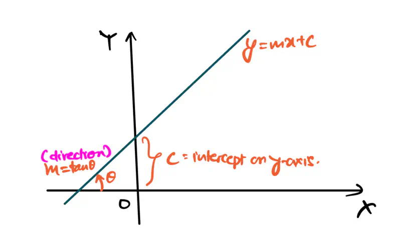
Similarly, to represent a hyperplane in d-dimensions, we need 2 things:
- \(\vec{w}\) = direction of the hyperplane = vector perpendicular to the hyperplane
- \(w_0\) = distance from the origin
Note: There can be only 2 directions of the hyperplane, i.e, direction of a unit vector perpendicular to the hyperplane:
- Towards the origin
- Away from the origin
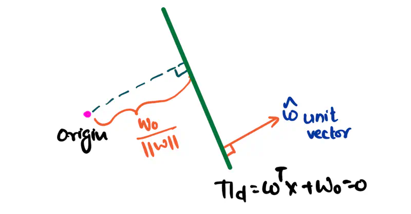
If a point ‘x’ is on the hyperplane, then it satisfies the below equation:
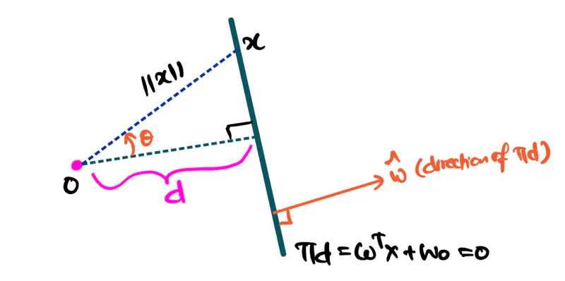
Key Points:
- By convention, the direction of the hyperplane is given by a unit vector perpendicular to the hyperplane , i.e, \({\Vert \mathbf{w} \Vert} = 1\), since the direction is only important.
- \(w_0\) gives the signed perpendicular distance from the origin.
\(w_0 = 0\) => Hyperplane passes through the origin.
\(w_0 < 0\) => Hyperplane is in the same direction of unit vector \(\mathbf{\widehat{w}}\) w.r.t the origin.
\(w_0 > 0\) => Hyperplane is in the opposite direction of unit vector \(\mathbf{\widehat{w}}\) w.r.t the origin.
What is the direction of the hyperplane w.r.t the origin and the direction of the unit vector ?
Equation of a hyperplane is: \(\pi_d = \mathbf{w}^\top \mathbf{x} + w_0 = 0\)
Let, the equation of the line/hyperplane in 2D be:
\(\pi_d = 1.x + 0.y + w_0 = x + w_0 = 0\)
Case 1: \(w_0 < 0\), say \(w_0 = -5\)
Therefore, equation of hyperplane: \( x - 5 = 0 => x = 5\)
Here, the hyperplane(line) is located in the same direction as the unit vector w.r.t the origin,
i.e, towards the +ve x-axis direction.
Case 2: \(w_0 > 0\), say \(w_0 = 5\)
Therefore, equation of hyperplane: \( x + 5 = 0 => x = -5\)
Here, the hyperplane(line) is located in the opposite direction as the unit vector w.r.t the origin,
i.e, towards the -ve x-axis direction.
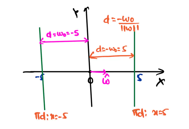
A hyperplane divides a space into 2 distinct parts called half-spaces.
e.g.: A 2D hyperplane divided a 3D space into 2 distinct parts.
Similar example in real world: A wall divides a room into 2 distinct spaces.
Positive Half-Space:
A half space that is in the same direction as the unit vector w.r.t the origin.
Negative Half-Space:
A half space that is in the opposite direction as the unit vector w.r.t the origin.
from equations (1) & (2), we can say that:
\[ \Vert \mathbf{w} \Vert \Vert \mathbf{x_1} \Vert cos{\theta} + w_0 < \Vert \mathbf{w} \Vert \Vert \mathbf{x_1\prime} \Vert cos{\theta} + w_0 \]Everything is same on both the sides except \(\Vert \mathbf{x_1}\Vert\) and \(\Vert \mathbf{x_1\prime\Vert}\), so:
\[ \mathbf{w}^\top \mathbf{x_1} + w_0 < 0 \]i.e, negative half-space, opposite to the direction of unit vector or towards the origin.
Similarly,
i.e, positive half-space, same as the direction of unit vector or away from the origin.
Equation of distance of any point \(x\prime\) from the hyperplane:
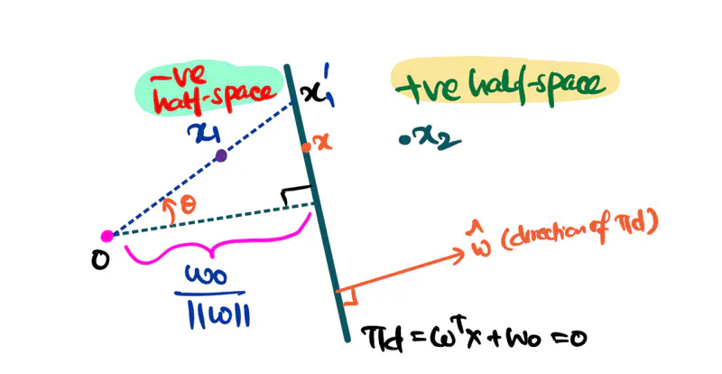
The above concept of equation of hyperplane will be very helpful when we discuss the following topics later:
- Logistic Regression
- Support Vector Machines
End of Section
4.1 - Calculus Fundamentals
Integration is a mathematical tool that is used to find the area under a curve.
Let’s understand integration with the help of few simple examples for finding area under a curve:
- Area of a triangle:
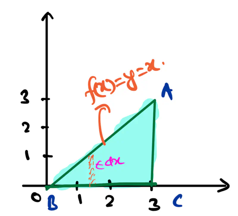
- Area of a rectangle:
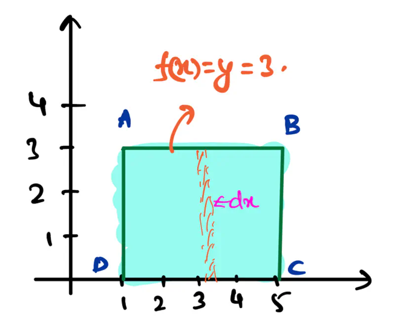
Note: The above examples were standard straight forward, where we know a direct formula for finding area under a curve.
But, what if we have such a shape, for which, we do NOT know a ready-made formula, then how do we calculate
the area under the curve.
Let’s see an example:
3. Area of a part of parabola:
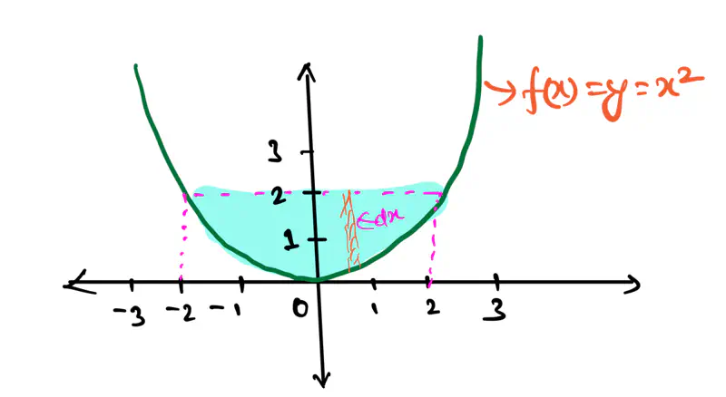
Differentiation is a mathematical tool that is used to find the derivative or rate of change of a function
at a specific point.
- \(\frac{dy}{dx} = f\prime(x) = tan\theta\) = Derivative = Slope = Gradient
- Derivative tells us how fast the function is changing at a specific point in relation to another variable.
Note: For a line, the slope is constant, but for a parabola, the slope is changing at every point.
How do we calculate the slope at a given point?
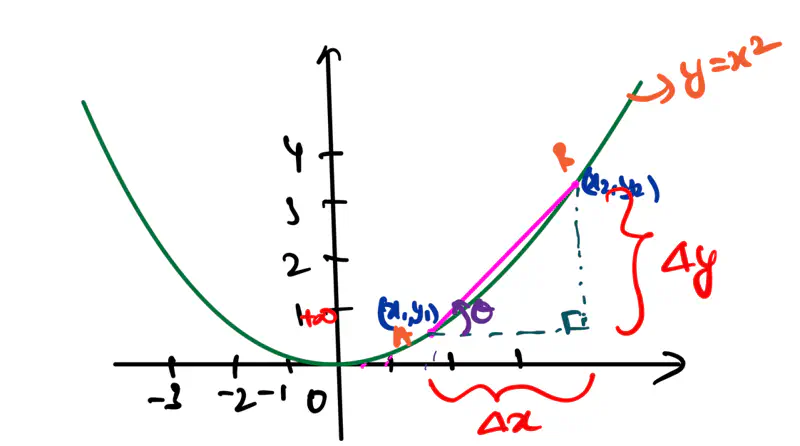
Let AB is a secant on the parabola, i.e, line connecting any 2 points on the curve.
Slope of secant = \(tan\theta = \frac{\Delta y}{\Delta x} = \frac{y_2-y_1}{x_2-x_1}\)
As \(\Delta x \rightarrow 0\), secant will become a tangent to the curve, i.e, the line will touch the curve only
at 1 point.
\(dx = \Delta x \rightarrow 0\)
\(x_2 = x_1 + \Delta x \)
\(y_2 = f(x_2) = f(x_1 + \Delta x) \)
Slope at \(x_1\) =
e.g.:
\( y = f(x) = x^2\), find the derivative of f(x) w.r.t x.
We will understand few important rules of differentiation that are most frequently used in Machine Learning.
Sum Rule:
\[ \frac{d}{dx} (f(x) + g(x)) = \frac{d}{dx} f(x) + \frac{d}{dx} g(x) = f\prime(x) + g\prime(x) \]Product Rule:
\[ \frac{d}{dx} (f(x).g(x)) = \frac{d}{dx} f(x).g(x) + f(x).\frac{d}{dx} g(x) = f\prime(x).g(x) + f(x).g\prime(x) \]e.g.:
\[ h(x) = f(x).g(x) \\[10pt] => h\prime(x) = f\prime(x).g(x) + f(x).g\prime(x) \\[10pt] => h\prime(x) = 2x.sin(x) + x^2.cos(x) \\[10pt] \]
\( h(x) = x^2 sin(x) \), find the derivative of h(x) w.r.t x.
Let, \(f(x) = x^2 , g(x) = sin(x)\).Quotient Rule:
\[ \frac{d}{dx} \frac{f(x)}{g(x)} = \frac{f\prime(x).g(x) - f(x).g\prime(x)}{(g(x))^2} \]e.g.:
\[ h(x) = \frac{f(x)}{g(x)} \\[10pt] => h\prime(x) = \frac{f\prime(x).g(x) - f(x).g\prime(x)}{(g(x))^2} \\[10pt] => h\prime(x) = \frac{cos(x).x - sin(x)}{x^2} \\[10pt] \]
\( h(x) = sin(x)/x \), find the derivative of h(x) w.r.t x.
Let, \(f(x) = sin(x) , g(x) = x\).Chain Rule:
\[ \frac{d}{dx} (f(g(x))) = f\prime(g(x)).g\prime(x) \]e.g.:
\[ h(x) = log(u) \\[10pt] => h\prime(x) = \frac{d h(x)}{du} \cdot \frac{du}{dx} \\[10pt] => h\prime(x) = \frac{1}{u} \cdot 2x = \frac{2x}{x^2} \\[10pt] => h\prime(x) = \frac{2}{x} \]
\( h(x) = log(x^2) \), find the derivative of h(x) w.r.t x.
Let, \( u = x^2 \)
Now, let’s dive deeper and understand the concepts that required for differentiation, such as, limits, continuity, differentiability, etc.
Limit of a function f(x) at any point ‘c’ is the value that f(x) approaches, as x gets very close to ‘c’,
but NOT necessarily equal to ‘c’.
One-sided limit: value of the function, as it approaches a point ‘c’ from only one direction, either left or right.
Two-sided limit: value of the function, as it approaches a point ‘c’ from both directions, left and right, simultaneously.
e.g.:
- \(f(x) = \frac{1}{x}\), find the limit of f(x) at x = 0.
Let’s check for one-sided limit at x=0:
\[ \lim_{x \rightarrow 0^+} \frac{1}{x} = + \infty \\[10pt] \lim_{x \rightarrow 0^-} \frac{1}{x} = - \infty \\[10pt] so, \lim_{x \rightarrow 0^+} \frac{1}{x} ⍯ \lim_{x \rightarrow 0^-} \frac{1}{x} \\[10pt] => \text{ limit does NOT exist at } x = 0. \]
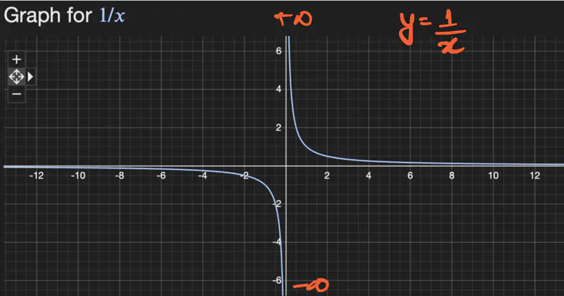
2. \(f(x) = x^2\), find the limit of f(x) at x = 0.
Let’s check for one-sided limit at x=0:
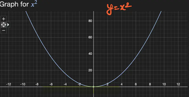
Note: Two-Sided Limit
3. f(x) = |x|, find the limit of f(x) at x = 0.
Let’s check for one-sided limit at x=0:
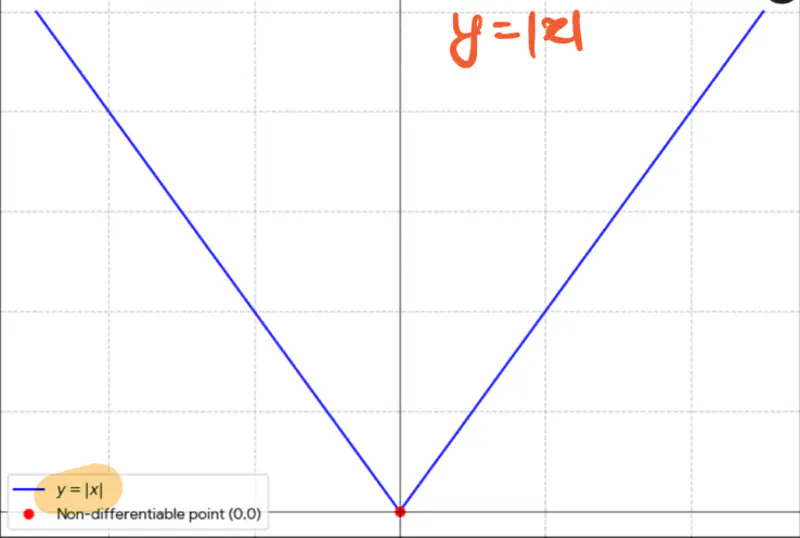
A function f(x) is said to be continuous at a point ‘c’, if its graph can be drawn through that point,
without lifting the pen.
Continuity bridges the gap between the function’s value at the given point and the limit.
Conditions for Continuity:
A function f(x) is continuous at a point ‘c’, if and only if, all the below 3 conditions are met:
- f(x) must be defined at point ‘c’.
- Limit of f(x) must exist at point ‘c’, i.e, left and right limits must be equal. \[ \lim_{x \rightarrow c^+} f(x) = \lim_{x \rightarrow c^-} f(x) \]
- Value of f(x) at ‘c’ must be equal to its limit at ‘c’. \[ \lim_{x \rightarrow c} f(x) = f(c) \]
e.g.:
- \(f(x) = \frac{1}{x}\) is NOT continuous at x = 0, since, f(x) is not defined at x = 0.
- \(f(x) = |x|\) is continuous everywhere.
- \(f(x) = tanx \) is discontinuous at infinite points.
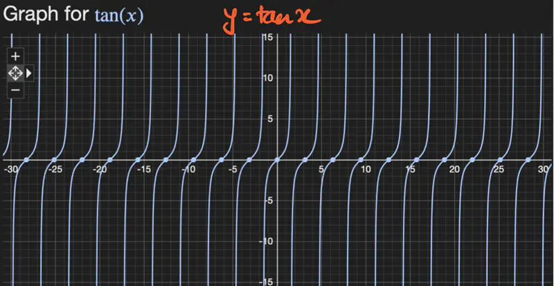
A function is differentiable at a point ‘c’, if derivative of the function exists at that point.
A function must be continuous at the given point ‘c’ to be differentiable at that point.
Note: A function can be continuous at a given point, but NOT differentiable at that point.
e.g.:
We know that \( f(x) = |x| \) is continuous at x=0, but its NOT differentiable at x=0.
Critical Point:
A point of the function where the derivative is either zero or undefined.
These critical points are candidates for local maxima or minima,
which are the highest and lowest points in a function’s immediate neighborhood, respectively.
Maxima:
Highest point w.r.t immediate neighbourhood.
f’(x)/gradient/slope changes from +ve to 0 to -ve, therefore, change in f’(x) is -ve.
=> f’’(x) < 0
Let, \(f(x) = -x^2; \quad f'(x) = -2x; \quad f''(x) = -2 < 0 => maxima\)
| x | f’(x) |
|---|---|
| -1 | 2 |
| 0 | 0 |
| 1 | -2 |
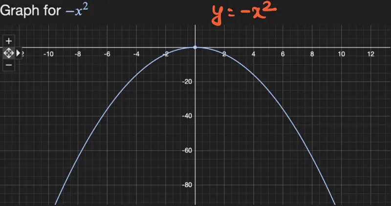
Minima:
Lowest point w.r.t immediate neighbourhood.
f’(x)/gradient/slope changes from -ve to 0 to +ve, therefore, change in f’(x) is +ve.
=> f’’(x) > 0
Let, \(f(x) = x^2; \quad f'(x) = 2x; \quad f''(x) = 2 > 0 => minima\)
| x | f’(x) |
|---|---|
| -1 | -2 |
| 0 | 0 |
| 1 | 2 |
e.g.:
- Let \(f(x) = 2x^3 + 5x^2 + 3 \), find the maxima and minima of f(x).
To find the maxima and minima, lets take the derivative of the function and equate it to zero.
\[ f'(x) = 6x^2 + 10x = 0\\[10pt] => x(6x+10) = 0 \\[10pt] => x = 0 \quad or \quad x = -10/6 = -5/3 \\[10pt] \text{ lets check the second order derivative to find which point is maxima and minima: } \\[10pt] f''(x) = 12x + 10 \\[10pt] => at ~ x = 0, \quad f''(x) = 12*0 + 10 = 10 >0 \quad => minima \\[10pt] => at ~ x = -5/3, \quad f''(x) = 12*(-5/3) + 10 = -20 + 10 = -10<0 \quad => maxima \\[10pt] \]
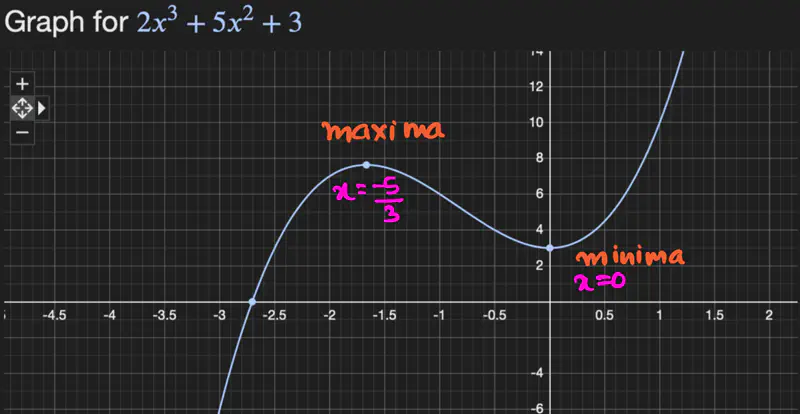
- \(f(x,y) = z = x^2 + y^2\), find the minima of f(x,y).
Since, this is a multi-variable function, we will use vector and matrix for calculation.
\[ Gradient = \nabla f_z = \begin{bmatrix} \frac{\partial f_z}{\partial x} \\ \\ \frac{\partial f_z}{\partial y} \end{bmatrix} = \begin{bmatrix} 2x \\ \\ 2y \end{bmatrix} = \begin{bmatrix} 0 \\ \\ 0 \end{bmatrix} \\[10pt] => x=0, y=0 \text{ is a point of optima for } f(x,y) \]
Partial Derivative:
Partial derivative \( \frac{\partial f(x,y)}{\partial x} ~or~ \frac{\partial f(x,y)}{\partial y} \)is the rate of change
or derivative of a multi-variable function w.r.t one of its variables,
while all the other variables are held constant.
Let’s continue solving the above problem, and calculate the Hessian, i.e, 2nd order derivative of f(x,y):
Since, determinant of Hessian = 4 > 0 and \( \frac{\partial^2 f_z}{\partial x^2} > 0\) => (x=0, y=0) is a point of minima.
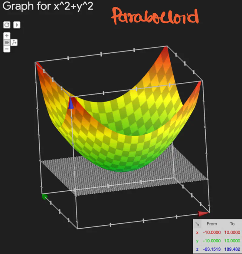
Hessian Interpretation:
- Minima: If det(Hessian) > 0 and \( \frac{\partial^2 f(x,y)}{\partial x^2} > 0\)
- Maxima: If det(Hessian) > 0 and \( \frac{\partial^2 f(x,y)}{\partial x^2} < 0\)
- Saddle Point: If det(Hessian) < 0
- Inconclusive: If det(Hessian) = 0, need to perform other tests.
Saddle Point is a critical point where the function is maximum w.r.t one variable,
and minimum w.r.t to another.
e.g.:
Let, \(f(x,y) = z = x^2 - y^2\), find the point of optima for f(x,y).
Since, determinant of Hessian = -4 < 0 => (x=0, y=0) is a saddle point.
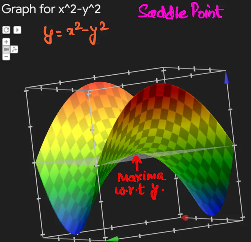
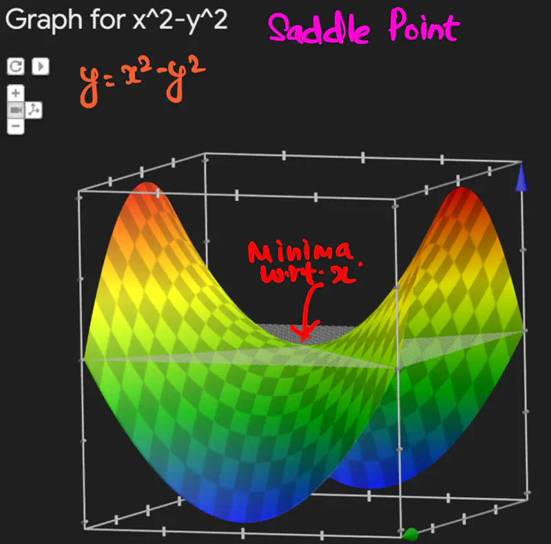
End of Section
4.2 - Optimization
How do we measure and minimize these mistakes in predictions made by the model?
minimizing a loss function.
Loss Function:
It quantifies error of a single data point in a dataset.
e.g.: Squared Loss, Hinge Loss, Absolute Loss, etc, for a single data point.
Cost Function:
It is the average of all losses over the entire dataset.
e.g.: Mean Squared Error(MSE), Mean Absolute Error(MAE), etc.
Objective Function:
It is the over-arching objective of an optimization problem, representing the function that is minimized or maximized.
e.g.: Minimize MSE.
Let’s understant this through an example:
Task:
Predict the price of a company’s stock based on its historical data.
Objective Function:
Minimize the difference between actual and predicted price.
Let, \(y\): original or actual price
\(\hat y\): predicted price
Say, the dataset has ’n’ such data points.
Loss Function:
loss = \( y - \hat y \) for a single data point.
We want to minimize the loss for all ’n’ data points.
Cost Function:
We want to minimize the average/total loss over all ’n’ data points.
So, what are the ways ?
- We take a simple sum of all the losses, but this can be misleading, as loss for a
single data point can be +ve or -ve, we can get a net-zero loss even for very large losses, when we sum them all. - We take the sum of absolute value of each loss, i.e, \( |y - \hat y| \), this way the losses will not cancel out each other.
But the absolute value function is NOT differentiable at y=0, and this can cause issues in optimisation algorithms, such as, gradient descent.
Read more about Differentiability - So, we choose squared loss, i.e, \( (y - \hat y)^2 \), this solves the above issues.
Note: In general, we refer to the cost function as the loss function also, the terms are used interchangeably.
Cost = Loss = Mean Squared Error(MSE) \[\frac{1}{n} \sum_{i=1}^{n} (y_i - \hat y_i)^2 \] The task is to minimize the above loss.
Key Points:
- Loss is the bridge between ‘data’ and ‘optimization’.
- Good loss functions are differentiable and convex.
Convexity:
It refers to a property of a function where a line segment connecting any two points on its graph
lies above or on the graph itself.
A convex function is curved upwards.
It is always described by a convex set.
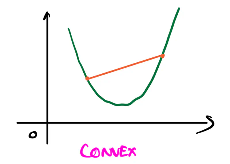
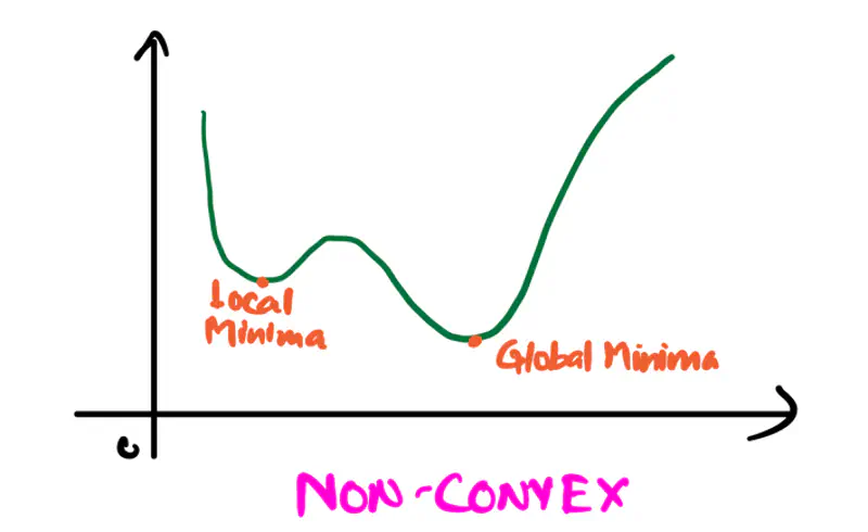
Convex Set:
A convex set is a set of points in which the straight line segment connecting any two points in the set lies
entirely within that set.
A set \(C\) is convex if for any two points \(x\) and \(y\) in \(C\), the convex combination
\(\theta x+(1-\theta )y\) is also in \(C\) for all values of \(\theta \) where \(0\le \theta \le 1\).
A function \(f: \mathbb{R}^n \rightarrow \mathbb{R}\) is convex if for all values of \(x,y\) and \(0\le \theta \le 1\),
\[ f(\theta x + (1-\theta )y) \le \theta f(x) + (1-\theta )f(y) \]Second-Order Test:
If a function is twice differentiable, i.e, 2nd derivative exists, then the function is convex,
if and only if, the Hessian is positive semi-definite for all points in its domain.
Positive Definite:
A symmetric matrix is positive definite if and only if:
- Eigenvalues are all strictly positive, or
- For any non-zero vector \(z\), the quadratic form \(z^THz > 0\)
Note: If the Hessian is positive definite, then the function is convex; has upward curvature in all directions.
Positive Semi-Definite:
A symmetric matrix is positive semi-definite if and only if:
- Eigenvalues are all non-negative (i.e, greater than or equal to zero), or
- For any non-zero vector \(z\), the quadratic form \(z^THz \ge 0\)
Note: If the Hessian is positive definite, then the function is not strictly convex, but flat in some directions.
All machine learning algorithms minimize loss (mostly), so we need to find the optimum parameters for the model that
minimizes the loss.
This is an optimization problem, i.e, find the best solution from a set of alternatives.
Note: Convexity ensures that there is only 1 minima for the loss function.
Optimization:
It is the iterative procedure of finding the optimum parameter \(x^*\) that minimizes the loss function f(x).
Let’s formulate an optimization problem for a model to minimize the MSE loss function discussed above:
Note: To minimize the loss, we want \(y_i, \hat y_i\) to be as close as possible, for that we want to find the optimum weights \(w, w_0\) of the model.
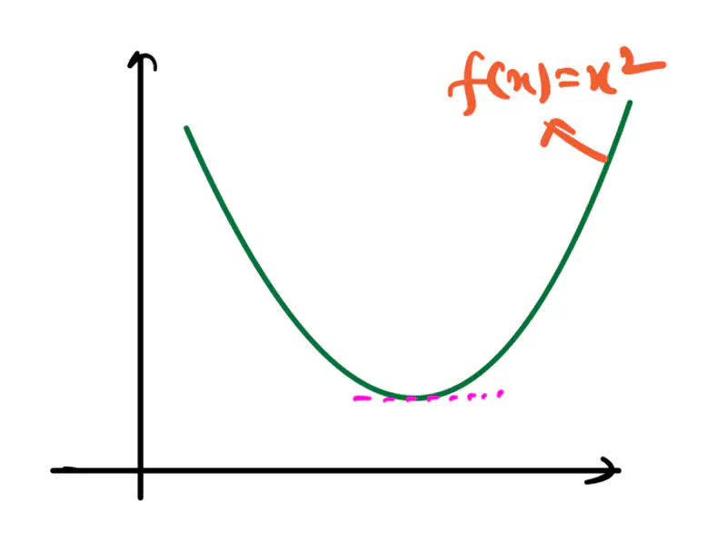
Important:
Deep Learning models have non-convex loss function, so it is challenging to reach the global minima,
so any local minima is also a good enough solution.
Read more about Maxima-Minima
Constrained Optimization:
It is an optimization process to find the best possible solution (min or max), but within a set of limitations or
restrictions called constraints.
Constraints limit the range of acceptable values; they can be equality constraints or inequality constraints.
e.g.:
Minimize f(x) subject to following constraints:
Equality Constraints: \( g_i(x) = c_i \forall ~i \in \{1,2,3, \ldots, n\} \)
Inequality Constraints: \( h_j(x) \le d_j \forall ~j \in \{1,2,3, \ldots, m\}\)
Lagrangian Method:
Lagrangian method converts a constrained optimization problem to an unconstrained optimization problem,
by introducing a new variable called Lagrange multiplier (\(\lambda\)).
Note: Addition of Lagrangian function that incorporates the constraints,
makes the problem solvable using standard calculus.
e.g.:
Let f(x) be the objective function with single equality constraint \(g(x) = c\),
then the Lagrangian function \( \mathcal{L}\) is defined as:
Now, the above constrained optimization problem becomes an unconstrained optimization problem:
By solving the above unconstrained optimization problem,
we get the optimum solution for the original constrained problem.
Objective: To minimize the distance between point (x,y) on the line 2x + 3y = 13 and the origin (0,0).
distance, d = \(\sqrt{(x-0)^2 + (y-0)^2}\)
=> Objective function = minimize distance = \( \underset{x^*, y^*}{\mathrm{argmin}}\ f(x,y) =
\underset{x^*, y^*}{\mathrm{argmin}}\ x^2+y^2\)
Constraint: Point (x,y) must be on the line 2x + 3y = 13.
=> Constraint (equality) function = \(g(x,y) = 2x + 3y - 13 = 0\)
Lagragian function =
To find the optimum solution, we solve the below unconstrained optimization problem.
Take the derivative and equate it to zero.
Since, it is multi-variable function, we take the partial derivatives, w.r.t, x, y and \(\lambda\).
Now, we have 3 variables and 3 equations (1), (2) and (3), lets solve them.
Hence, the point (x=2, y=3) on the line 2x + 3y = 13 that is closest to the origin.
To solve the optimization problem, there are many methods, such as, analytical method, which gives the normal equation for the linear regression,
but we will discuss that method later in detail, when we have understood what is linear regression?
Normal Equation for linear regression:
X: Feature variables
y: Vector of all observed target values
End of Section
4.3 - Gradient Descent
Till now, we have understood how to formulate a minimization problem as a mathematical optimization problem.
Now, lets take a step forward and understand how to solve these optimization problems.
We will focus on two important iterative gradient based methods:
- Gradient Descent: First order method, uses only the gradient.
- Newton’s Method: Second order method, used both the gradient and the Hessian.
Gradient Descent:
It is a first order iterative optimization algorithm that is used to find the local minimum of a differentiable function.
It iteratively adjusts the parameters of the model in the direction opposite to the gradient of cost function,
since moving opposite to the direction of gradient leads towards the minima.
Algorithm:
Initialize the weights/parameters with random values.
Calculate the gradient of the cost function at current parameter values.
Update the parameters using the gradient.
\[ w_{new} = w_{old} - \eta \cdot \frac{\partial f}{\partial w_{old}} \\[10pt] \eta: \text{ learning rate or step size to take for each parameter update} \]Repeat steps 2 and 3 iteratively until convergence (to minima).
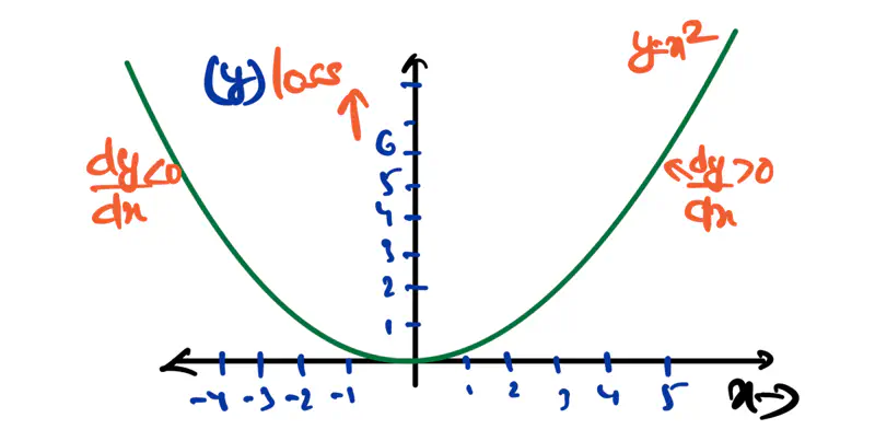
There are 3 types of Gradient Descent:
- Batch Gradient Descent
- Stochastic Gradient Descent
- Mini-Batch Gradient Descent
Batch Gradient Descent (BGD):
Computes the gradient using all the data points in the dataset for parameter update in each iteration.
Say, number of data points in the dataset is \(n\).
Let, the loss function for individual data point be \(l_i(w)\)
Key Points:
- Slow steps towards convergence, i.e, TC = O(n).
- Smooth, direct path towards minima.
- Number of steps/iterations is minimum.
- Not suitable for large datasets; impractical for Deep Learning, as n = millions/billions.
Stochastic Gradient Descent (SGD):
It uses only 1 data point selected randomly from dataset to compute gradient for parameter update in each iteration.
Key Points:
- Computationally fastest per step; TC = O(1).
- Highly noisy, zig-zag path to minima.
- High variance in gradient estimation makes path to minima volatile, requiring a careful decay of learning rate \(\eta\) to ensure convergence to minima.
Mini Batch Gradient Descent (MBGD):
It uses small randomly selected subsets of dataset, called mini-batch, (1<k<n) to compute gradient for
parameter update in each iteration.
Key Points:
- Moderate time consumption per step; TC = O(k<n).
- Less noisy, and more reliable convergence than stochastic gradient descent.
- More efficient and faster than batch gradient descent.
- Standard optimization algorithm for Deep Learning.
Note: Vectorization on GPUs allows for parallel processing of mini-batches; also GPUs are the reason for the mini-batch size to be a power of 2.
End of Section
4.4 - Newton's Method
Newton’s Method:
It is a second-order iterative gradient based optimization technique known for its extremely fast convergence.
When close to optimum, it achieves quadratic convergence, better than gradient descent’s linear convergence.
Algorithm:
- Start at a random point \(x_k\).
- Compute the slope at \(x_k, ~i.e,~ f'(x_k)\).
- Compute the curvature at \(x_k, ~i.e,~ f''(x_k)\).
- Draw a parabola at \(x_k\) that locally approximates the function.
- Jump directly to the minimum of that parabola; that’s the next step. Note: So, instead of walking down the slope step by step (gradient descent), we are jumping straight to the point where the curve bends downwards towards the bottom.
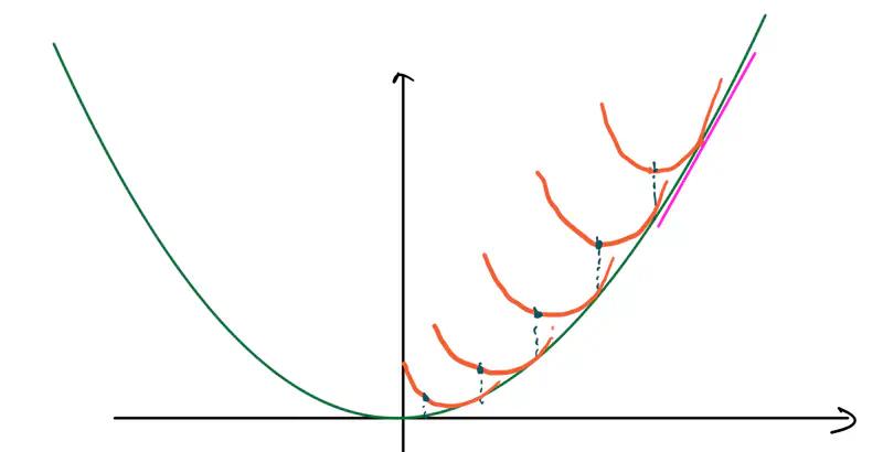
- Find the minima of \(f(x) = x^2 - 4x + 5\)
To find the minima, lets calulate the first derivative and equate to zero.
\(f'(x) = 2x - 4 = 0 \)
\( => x^* = 2 \)
\(f''(x) = 2 >0 \) => minima is at \(x^* = 2\)
Now, we will solve this using Newton’s Method.
Let’s start at x = 0.
Hence, we can see that using Newton’s Method we can get to the minima \(x^* = 2\) in just 1 step.
Full Newton’s Method is rarely used in Machine Learning/Deep Learning optimization,
because of the following limitations:
- \(TC = O(n^2\)) for Hessian calculation, since for a network with \(n\) parameters
requires \(n^2\) derivative calculations. - \(TC = O(n^3\)) for Hessian Inverse calculation.
- If it encounters a Saddle point, then it can go to a maxima rather than minima.
Because of the above limitations, we use Quasi-Newton methods like BFGS and L-BFGS.
The quasi-Newton methods make use of approximations for Hessian calculation, in order to gain the benefits
of curvature without incurring the cost of Hessian calculation.
BFGS: Broyden-Fletcher-Goldfarb-Shanno
L-BFGS: Limited-memory BFGS
End of Section