This is the multi-page printable view of this section. Click here to print.

Return to the regular view of this page.

Calculus

Calculus for AI & ML

1: Calculus Fundamentals
2: Optimization
3: Gradient Descent
4: Newton's Method

Calculus for AI & ML | Full Course Videos

Calculus for AI & ML

This sheet contains all the topics that will be covered for Calculus for AI & ML.

1 - Calculus Fundamentals

Calculus Fundamentals

Calculus for AI & ML | Full Course Videos

Integration

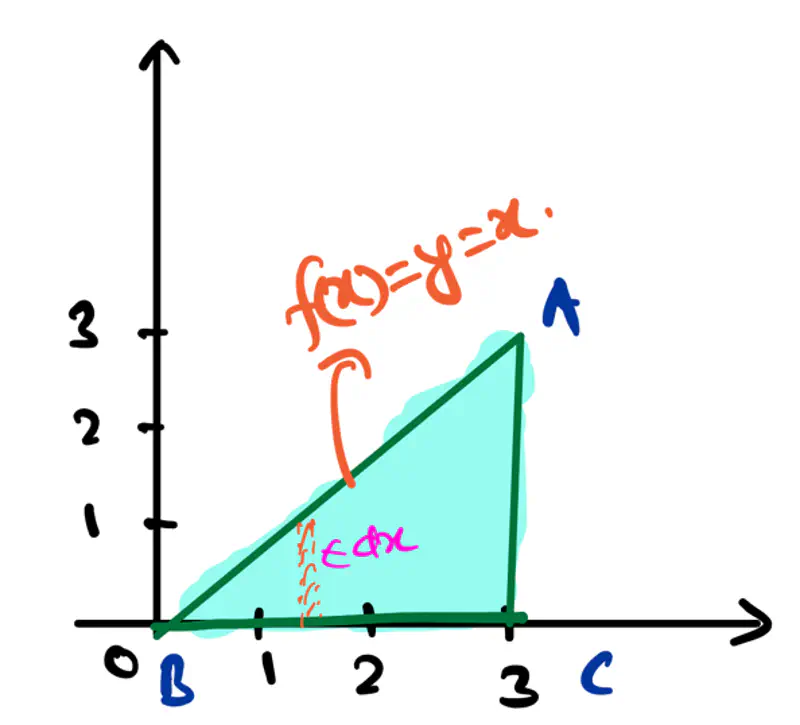
Integration is a mathematical tool that is used to find the area under a curve.

\[ \text{Area under the curve = } \int_{a}^{b} f(x) dx \\[10pt] and ~ \int x^n dx = \frac{x^{n+1}}{n+1} + C, \text{ where C is constant.} \\ \]

Let’s understand integration with the help of few simple examples for finding area under a curve:

Area of a triangle:
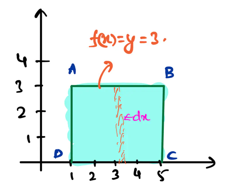
\[ \text{Area of } \triangle ~ABC = \frac{1}{2} \times base \times height = \frac{1}{2} \times 3 \times 3 = 9/2 = 4.5 \\[10pt] \text{Area of } \triangle ~ABC = \int_0^3 f(x) dx = \int_0^3 x dx = \frac{x^2}{2} \big|_0^3 = \frac{3^2 - 0^2}{2} = 9/2 = 4.5 \]
Area of a rectangle:
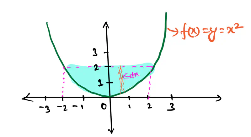
\[ \text{Area of rectangle ABCD} = length \times breadth = 4 \times 3 = 12 \\[10pt] \text{Area of rectangle ABCD} = \int_1^5 f(x) dx = \int_1^5 3 dx = 3x \big|_1^5 = 3(5-1) = 12 \]

Note: The above examples were standard straight forward, where we know a direct formula for finding area under a curve.
But, what if we have such a shape, for which, we do NOT know a ready-made formula, then how do we calculate the area under the curve.
Let’s see an example:

3. Area of a part of parabola:

\[ \text{Area under curve} = \int_{-2}^2 f(x) dx = \int_{-2}^2 x^2 dx = \frac{x^3}{3} \big|_{-2}^2 = \frac{(2)^3 - (-2)^3}{3} = \frac{8 - (-8)}{3} = \frac{16}{3} \]

Watch Video

Differentiation

Differentiation is a mathematical tool that is used to find the derivative or rate of change of a function at a specific point.

\(\frac{dy}{dx} = f\prime(x) = tan\theta\) = Derivative = Slope = Gradient
Derivative tells us how fast the function is changing at a specific point in relation to another variable.

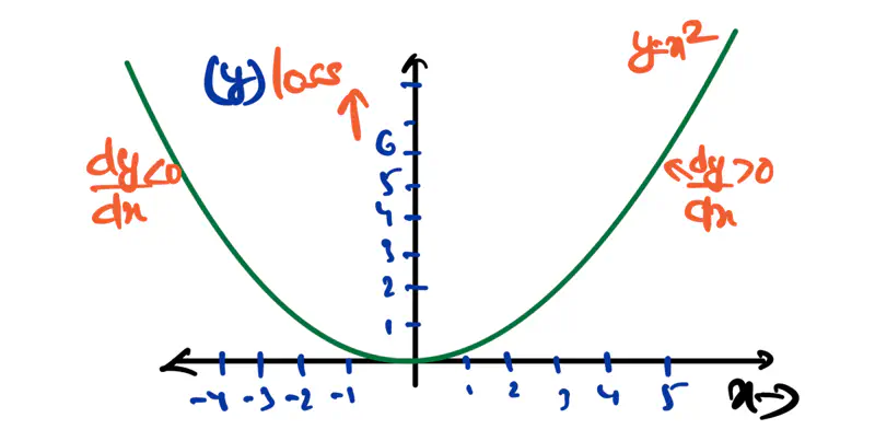
Note: For a line, the slope is constant, but for a parabola, the slope is changing at every point.

How do we calculate the slope at a given point?

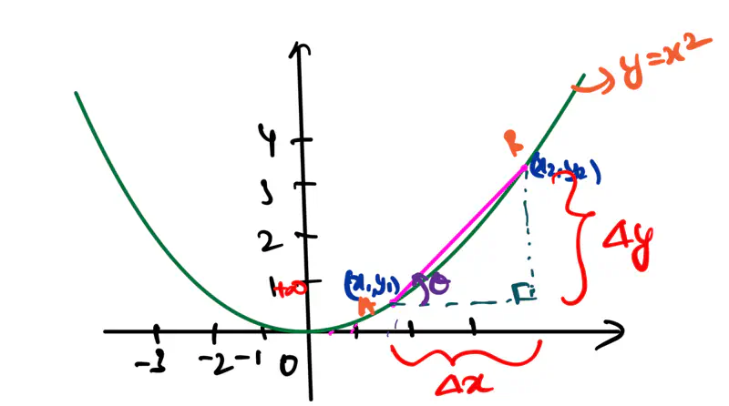
Let AB is a secant on the parabola, i.e, line connecting any 2 points on the curve.
Slope of secant = \(tan\theta = \frac{\Delta y}{\Delta x} = \frac{y_2-y_1}{x_2-x_1}\)
As \(\Delta x \rightarrow 0\), secant will become a tangent to the curve, i.e, the line will touch the curve only at 1 point.
\(dx = \Delta x \rightarrow 0\)
\(x_2 = x_1 + \Delta x \)
\(y_2 = f(x_2) = f(x_1 + \Delta x) \)
Slope at \(x_1\) =

\[ tan \theta = \frac{y_2-y_1}{x_2-x_1} = \frac{f(x_1 + \Delta x) - f(x_1)}{(x_1 + \Delta x)-x_1} \\[10pt] \therefore tan \theta = \lim_{\Delta x \rightarrow 0} \frac{f(x_1 + \Delta x) - f(x_1)}{\Delta x} \\[10pt] Generally, ~ slope = ~ tan \theta = \frac{dy}{dx} = \lim_{\Delta x \rightarrow 0} \frac{f(x + \Delta x) - f(x)}{\Delta x} \]

e.g.:
\( y = f(x) = x^2\), find the derivative of f(x) w.r.t x.

\[ \begin{aligned} \frac{dy}{dx} &= \lim_{\Delta x \rightarrow 0} \frac{f(x + \Delta x) - f(x)}{\Delta x} \\[10pt] &= \lim_{\Delta x \rightarrow 0} \frac{(x + \Delta x)^2 - x^2}{\Delta x} \\[10pt] &= \lim_{\Delta x \rightarrow 0} \frac{\cancel {x^2} + (\Delta x)^2 + 2x\Delta x - \cancel {x^2}}{\Delta x} \\[10pt] &= \lim_{\Delta x \rightarrow 0} \frac{\cancel {\Delta x}(\Delta x + 2x)}{\cancel {\Delta x}} \\[10pt] \text {applying limit: } \\ \therefore \frac{dy}{dx} &= 2x \\[10pt] \end{aligned} \]

Rules of Differentiation

We will understand few important rules of differentiation that are most frequently used in Machine Learning.

Sum Rule:
\[ \frac{d}{dx} (f(x) + g(x)) = \frac{d}{dx} f(x) + \frac{d}{dx} g(x) = f\prime(x) + g\prime(x) \]
Product Rule:
\[ \frac{d}{dx} (f(x).g(x)) = \frac{d}{dx} f(x).g(x) + f(x).\frac{d}{dx} g(x) = f\prime(x).g(x) + f(x).g\prime(x) \]
e.g.:
\( h(x) = x^2 sin(x) \), find the derivative of h(x) w.r.t x.
Let, \(f(x) = x^2 , g(x) = sin(x)\).
\[ h(x) = f(x).g(x) \\[10pt] => h\prime(x) = f\prime(x).g(x) + f(x).g\prime(x) \\[10pt] => h\prime(x) = 2x.sin(x) + x^2.cos(x) \\[10pt] \]
Quotient Rule:
\[ \frac{d}{dx} \frac{f(x)}{g(x)} = \frac{f\prime(x).g(x) - f(x).g\prime(x)}{(g(x))^2} \]
e.g.:
\( h(x) = sin(x)/x \), find the derivative of h(x) w.r.t x.
Let, \(f(x) = sin(x) , g(x) = x\).
\[ h(x) = \frac{f(x)}{g(x)} \\[10pt] => h\prime(x) = \frac{f\prime(x).g(x) - f(x).g\prime(x)}{(g(x))^2} \\[10pt] => h\prime(x) = \frac{cos(x).x - sin(x)}{x^2} \\[10pt] \]
Chain Rule:
\[ \frac{d}{dx} (f(g(x))) = f\prime(g(x)).g\prime(x) \]
e.g.:
\( h(x) = log(x^2) \), find the derivative of h(x) w.r.t x.
Let, \( u = x^2 \)
\[ h(x) = log(u) \\[10pt] => h\prime(x) = \frac{d h(x)}{du} \cdot \frac{du}{dx} \\[10pt] => h\prime(x) = \frac{1}{u} \cdot 2x = \frac{2x}{x^2} \\[10pt] => h\prime(x) = \frac{2}{x} \]

Now, let’s dive deeper and understand the concepts that required for differentiation, such as, limits, continuity, differentiability, etc.

Limits

Limit of a function f(x) at any point ‘c’ is the value that f(x) approaches, as x gets very close to ‘c’,
but NOT necessarily equal to ‘c’.

One-sided limit: value of the function, as it approaches a point ‘c’ from only one direction, either left or right.
Two-sided limit: value of the function, as it approaches a point ‘c’ from both directions, left and right, simultaneously.

e.g.:

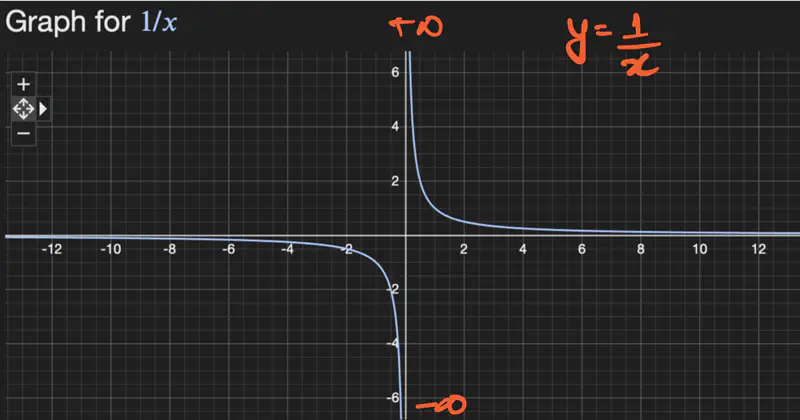
\(f(x) = \frac{1}{x}\), find the limit of f(x) at x = 0.
Let’s check for one-sided limit at x=0:
\[ \lim_{x \rightarrow 0^+} \frac{1}{x} = + \infty \\[10pt] \lim_{x \rightarrow 0^-} \frac{1}{x} = - \infty \\[10pt] so, \lim_{x \rightarrow 0^+} \frac{1}{x} ⍯ \lim_{x \rightarrow 0^-} \frac{1}{x} \\[10pt] => \text{ limit does NOT exist at } x = 0. \]
\(f(x) = x^2\), find the limit of f(x) at x = 0.
Let’s check for one-sided limit at x=0:
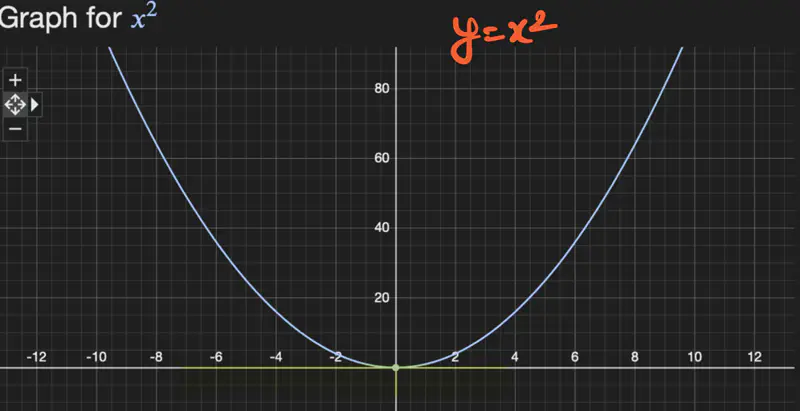
\[ \lim_{x \rightarrow 0^+} x^2 = 0 \\[10pt] \lim_{x \rightarrow 0^-} x^2 = 0 \\[10pt] so, \lim_{x \rightarrow 0^+} x^2 = \lim_{x \rightarrow 0^-} x^2 \\[10pt] => \text{ limit exists at } x = 0. \]

Note: Two-Sided Limit
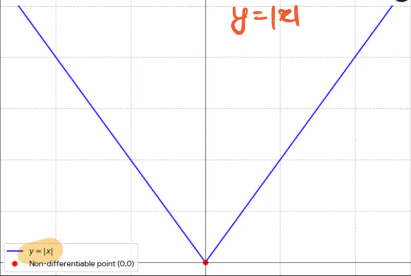
\[ \lim_{x \rightarrow a^+} f(x) = \lim_{x \rightarrow a^-} f(x) = \lim_{x \rightarrow a} f(x) \]
f(x) = |x|, find the limit of f(x) at x = 0.
Let’s check for one-sided limit at x=0:
\[ \lim_{x \rightarrow 0^+} |x| = x = 0 \\[10pt] \lim_{x \rightarrow 0^-} |x| = -x = 0 \\[10pt] so, \lim_{x \rightarrow 0^+} |x| = \lim_{x \rightarrow 0^-} |x| \\[10pt] => \text{ limit exists at } x = 0. \]

Continuity

A function f(x) is said to be continuous at a point ‘c’, if its graph can be drawn through that point, without lifting the pen.
Continuity bridges the gap between the function’s value at the given point and the limit.

Conditions for Continuity:
A function f(x) is continuous at a point ‘c’, if and only if, all the below 3 conditions are met:

f(x) must be defined at point ‘c’.
Limit of f(x) must exist at point ‘c’, i.e, left and right limits must be equal. \[ \lim_{x \rightarrow c^+} f(x) = \lim_{x \rightarrow c^-} f(x) \]
Value of f(x) at ‘c’ must be equal to its limit at ‘c’. \[ \lim_{x \rightarrow c} f(x) = f(c) \]

e.g.:

\(f(x) = \frac{1}{x}\) is NOT continuous at x = 0, since, f(x) is not defined at x = 0.
\(f(x) = |x|\) is continuous everywhere.
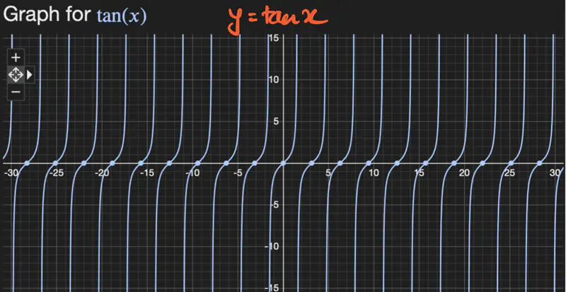
\(f(x) = tanx \) is discontinuous at infinite points.

Differentiability

A function is differentiable at a point ‘c’, if derivative of the function exists at that point.
A function must be continuous at the given point ‘c’ to be differentiable at that point.
Note: A function can be continuous at a given point, but NOT differentiable at that point.

\[ f\prime(x) = \lim_{\Delta x \rightarrow 0} \frac{f(x + \Delta x) - f(x)}{\Delta x} \]

e.g.:
We know that \( f(x) = |x| \) is continuous at x=0, but its NOT differentiable at x=0.

\[ f\prime(x) =\lim_{\Delta x \rightarrow 0} \frac{f(x + \Delta x) - f(x)}{\Delta x} = \lim_{\Delta x \rightarrow 0} \frac{|x + \Delta x| - |x|}{\Delta x} \\[10pt] \text{ let's calculate the one-sided limit from both left and right sides and check if they are equal: } \\[10pt] if ~ x>0, \lim_{\Delta x \rightarrow 0^+} \frac{|x + \Delta x| - |x|}{\Delta x} = \lim_{\Delta x \rightarrow 0+} \frac{\cancel x + \Delta x - \cancel x}{\Delta x} = 1 \\[10pt] if ~ x<0, \lim_{\Delta x \rightarrow 0^-} \frac{|x + \Delta x| - |x|}{\Delta x} = \lim_{\Delta x \rightarrow 0^-} \frac{-(x + \Delta x) - (-x)}{\Delta x} = \lim_{\Delta x \rightarrow 0-} \frac{\cancel {-x} - \Delta x + \cancel x}{\Delta x} = -1 \\[10pt] => \text{ left hand limit (-1) ⍯ right hand limit (1) } \\[10pt] => f\prime(0) \text{ does NOT exist.} \]

Maxima & Minima

Critical Point:
A point of the function where the derivative is either zero or undefined.

These critical points are candidates for local maxima or minima, which are the highest and lowest points in a function’s immediate neighborhood, respectively.

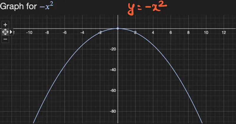
Maxima:
Highest point w.r.t immediate neighbourhood.
f’(x)/gradient/slope changes from +ve to 0 to -ve, therefore, change in f’(x) is -ve.
=> f’’(x) < 0

Let, \(f(x) = -x^2; \quad f'(x) = -2x; \quad f''(x) = -2 < 0 => maxima\)

x	f’(x)
-1	2
0	0
1	-2

Minima:
Lowest point w.r.t immediate neighbourhood.
f’(x)/gradient/slope changes from -ve to 0 to +ve, therefore, change in f’(x) is +ve.
=> f’’(x) > 0

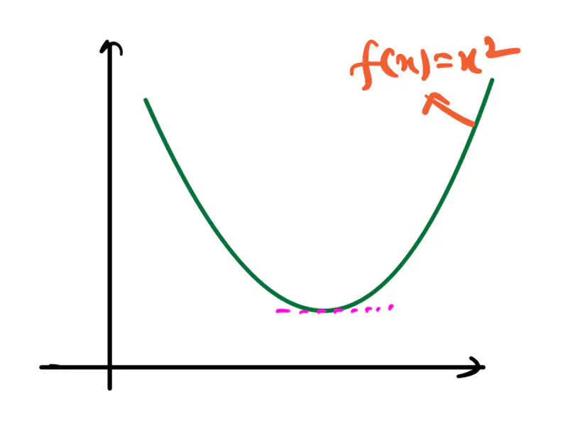
Let, \(f(x) = x^2; \quad f'(x) = 2x; \quad f''(x) = 2 > 0 => minima\)

x	f’(x)
-1	-2
0	0
1	2

e.g.:

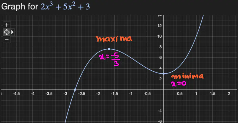
Let \(f(x) = 2x^3 + 5x^2 + 3 \), find the maxima and minima of f(x).
To find the maxima and minima, lets take the derivative of the function and equate it to zero.
\[ f'(x) = 6x^2 + 10x = 0\\[10pt] => x(6x+10) = 0 \\[10pt] => x = 0 \quad or \quad x = -10/6 = -5/3 \\[10pt] \text{ lets check the second order derivative to find which point is maxima and minima: } \\[10pt] f''(x) = 12x + 10 \\[10pt] => at ~ x = 0, \quad f''(x) = 12*0 + 10 = 10 >0 \quad => minima \\[10pt] => at ~ x = -5/3, \quad f''(x) = 12*(-5/3) + 10 = -20 + 10 = -10<0 \quad => maxima \\[10pt] \]
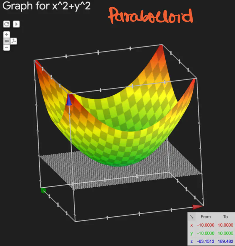
\(f(x,y) = z = x^2 + y^2\), find the minima of f(x,y).
Since, this is a multi-variable function, we will use vector and matrix for calculation.
\[ Gradient = \nabla f_z = \begin{bmatrix} \frac{\partial f_z}{\partial x} \\ \\ \frac{\partial f_z}{\partial y} \end{bmatrix} = \begin{bmatrix} 2x \\ \\ 2y \end{bmatrix} = \begin{bmatrix} 0 \\ \\ 0 \end{bmatrix} \\[10pt] => x=0, y=0 \text{ is a point of optima for } f(x,y) \]

Partial Derivative:
Partial derivative \( \frac{\partial f(x,y)}{\partial x} ~or~ \frac{\partial f(x,y)}{\partial y} \)is the rate of change or derivative of a multi-variable function w.r.t one of its variables, while all the other variables are held constant.

Let’s continue solving the above problem, and calculate the Hessian, i.e, 2nd order derivative of f(x,y):

\[ Hessian = H_z = \begin{bmatrix} \frac{\partial^2 f_z}{\partial x^2} & \frac{\partial^2 f_z}{\partial x \partial y} \\ \\ \frac{\partial^2 f_z}{\partial y \partial x} & \frac{\partial^2 f_z}{\partial y^2} \end{bmatrix} = \begin{bmatrix} 2 & 0 \\ \\ 0 & 2 \end{bmatrix} \]

Since, determinant of Hessian = 4 > 0 and \( \frac{\partial^2 f_z}{\partial x^2} > 0\) => (x=0, y=0) is a point of minima.

Hessian Interpretation:

Minima: If det(Hessian) > 0 and \( \frac{\partial^2 f(x,y)}{\partial x^2} > 0\)
Maxima: If det(Hessian) > 0 and \( \frac{\partial^2 f(x,y)}{\partial x^2} < 0\)
Saddle Point: If det(Hessian) < 0
Inconclusive: If det(Hessian) = 0, need to perform other tests.

Saddle Point

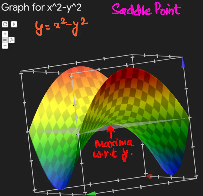
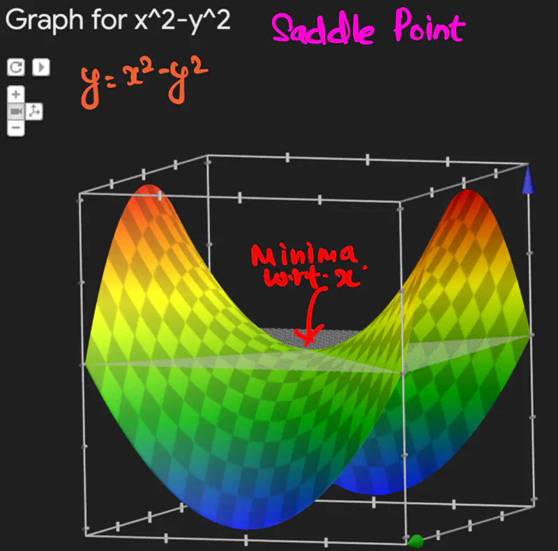
Saddle Point is a critical point where the function is maximum w.r.t one variable,
and minimum w.r.t to another.

e.g.:
Let, \(f(x,y) = z = x^2 - y^2\), find the point of optima for f(x,y).

\[ Gradient = \nabla f_z = \begin{bmatrix} \frac{\partial f_z}{\partial x} \\ \\ \frac{\partial f_z}{\partial y} \end{bmatrix} = \begin{bmatrix} 2x \\ \\ -2y \end{bmatrix} = \begin{bmatrix} 0 \\ \\ 0 \end{bmatrix} \\[10pt] => x=0, y=0 \text{ is a point of optima for } f(x,y) \]\[ Hessian = H_z = \begin{bmatrix} \frac{\partial^2 f_z}{\partial x^2} & \frac{\partial^2 f_z}{\partial x \partial y} \\ \\ \frac{\partial^2 f_z}{\partial y \partial x} & \frac{\partial^2 f_z}{\partial y^2} \end{bmatrix} = \begin{bmatrix} 2 & 0 \\ \\ 0 & -2 \end{bmatrix} \]

Since, determinant of Hessian = -4 < 0 => (x=0, y=0) is a saddle point.

Watch Video

End of Section

2 - Optimization

Loss Function, Convexity & Optimization

Calculus for AI & ML | Full Course Videos

💡 Whenever we build a Machine Learning model, we try to make sure that the model makes least mistakes in its predictions.
How do we measure and minimize these mistakes in predictions made by the model?

To measure, how wrong the are the predictions made by a Machine Learning model, every model is formulated as
minimizing a loss function.

Loss Function

Loss Function:
It quantifies error of a single data point in a dataset.
e.g.: Squared Loss, Hinge Loss, Absolute Loss, etc, for a single data point.

Cost Function:
It is the average of all losses over the entire dataset.
e.g.: Mean Squared Error(MSE), Mean Absolute Error(MAE), etc.

Objective Function:
It is the over-arching objective of an optimization problem, representing the function that is minimized or maximized.
e.g.: Minimize MSE.

Let’s understant this through an example:
Task:
Predict the price of a company’s stock based on its historical data.

Objective Function:
Minimize the difference between actual and predicted price.
Let, \(y\): original or actual price
\(\hat y\): predicted price

Say, the dataset has ’n’ such data points.
Loss Function:
loss = \( y - \hat y \) for a single data point.
We want to minimize the loss for all ’n’ data points.

Cost Function:
We want to minimize the average/total loss over all ’n’ data points.
So, what are the ways ?

We take a simple sum of all the losses, but this can be misleading, as loss for a
single data point can be +ve or -ve, we can get a net-zero loss even for very large losses, when we sum them all.
We take the sum of absolute value of each loss, i.e, \( |y - \hat y| \), this way the losses will not cancel out each other.
But the absolute value function is NOT differentiable at y=0, and this can cause issues in optimisation algorithms, such as, gradient descent.
Read more about Differentiability
So, we choose squared loss, i.e, \( (y - \hat y)^2 \), this solves the above issues.

Note: In general, we refer to the cost function as the loss function also, the terms are used interchangeably.

Cost = Loss = Mean Squared Error(MSE) \[\frac{1}{n} \sum_{i=1}^{n} (y_i - \hat y_i)^2 \] The task is to minimize the above loss.

Key Points:

Loss is the bridge between ‘data’ and ‘optimization’.
Good loss functions are differentiable and convex.

Convexity

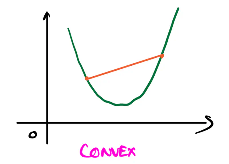
Convexity:
It refers to a property of a function where a line segment connecting any two points on its graph lies above or on the graph itself.
A convex function is curved upwards.
It is always described by a convex set.

Convex Set:
A convex set is a set of points in which the straight line segment connecting any two points in the set lies entirely within that set.
A set \(C\) is convex if for any two points \(x\) and \(y\) in \(C\), the convex combination
\(\theta x+(1-\theta )y\) is also in \(C\) for all values of \(\theta \) where \(0\le \theta \le 1\).

A function \(f: \mathbb{R}^n \rightarrow \mathbb{R}\) is convex if for all values of \(x,y\) and \(0\le \theta \le 1\),

\[ f(\theta x + (1-\theta )y) \le \theta f(x) + (1-\theta )f(y) \]

Second-Order Test:
If a function is twice differentiable, i.e, 2nd derivative exists, then the function is convex, if and only if, the Hessian is positive semi-definite for all points in its domain.

Optimization

All machine learning algorithms minimize loss (mostly), so we need to find the optimum parameters for the model that minimizes the loss.
This is an optimization problem, i.e, find the best solution from a set of alternatives.
Note: Convexity ensures that there is only 1 minima for the loss function.

Optimization:
It is the iterative procedure of finding the optimum parameter \(x^*\) that minimizes the loss function f(x).

\[ x^* = \underset{x}{\mathrm{argmin}}\ f(x) \]

Let’s formulate an optimization problem for a model to minimize the MSE loss function discussed above:

\[ Loss = \frac{1}{n} \sum_{i=1}^{n} (y_i - \hat y_i)^2 \\[10pt] \text { We need to find the weights } w, w_0 \text{ of the model that minimize our MSE loss: } \\[10pt] \underset{w, w_0}{\mathrm{argmin}}\ \frac{1}{n} \sum_{i=1}^{n} (y_i - \hat y_i)^2 \]

Note: To minimize the loss, we want \(y_i, \hat y_i\) to be as close as possible, for that we want to find the optimum weights \(w, w_0\) of the model.

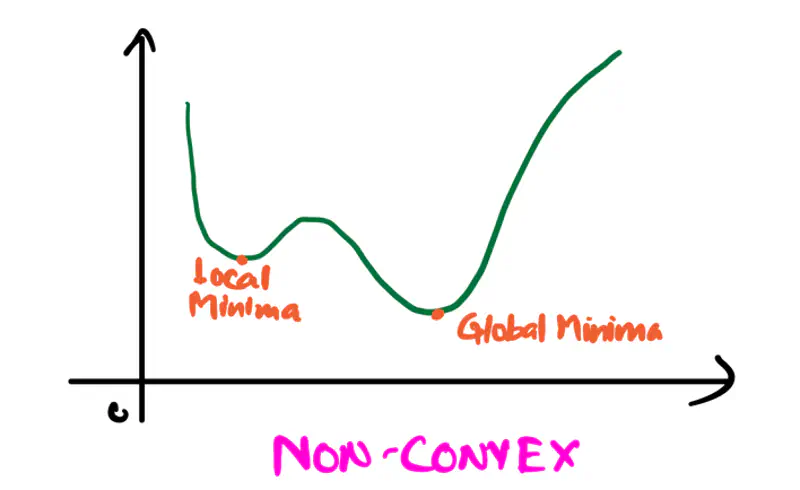
Important:
Deep Learning models have non-convex loss function, so it is challenging to reach the global minima, so any local minima is also a good enough solution.

Read more about Maxima-Minima

Constrained Optimization

Constrained Optimization:
It is an optimization process to find the best possible solution (min or max), but within a set of limitations or restrictions called constraints.
Constraints limit the range of acceptable values; they can be equality constraints or inequality constraints.
e.g.:
Minimize f(x) subject to following constraints:
Equality Constraints: \( g_i(x) = c_i \forall ~i \in \{1,2,3, \ldots, n\} \)
Inequality Constraints: \( h_j(x) \le d_j \forall ~j \in \{1,2,3, \ldots, m\}\)

Lagrangian Method:
Lagrangian method converts a constrained optimization problem to an unconstrained optimization problem, by introducing a new variable called Lagrange multiplier (\(\lambda\)).

Note: Addition of Lagrangian function that incorporates the constraints, makes the problem solvable using standard calculus.

e.g.:
Let f(x) be the objective function with single equality constraint \(g(x) = c\),
then the Lagrangian function \( \mathcal{L}\) is defined as:

\[ \mathcal {L}(\lambda, x) = f(x) - \lambda(g(x) - c) \]

Now, the above constrained optimization problem becomes an unconstrained optimization problem:

\[ \underset{x^*}{\mathrm{argmin}}\ \mathcal{L}(\lambda, x) = \underset{x^*}{\mathrm{argmin}}\ f(x) - \lambda(g(x) - c) \]

By solving the above unconstrained optimization problem, we get the optimum solution for the original constrained problem.

💡 Find the point on the line 2x + 3y = 13 that is closest to the origin.

Objective: To minimize the distance between point (x,y) on the line 2x + 3y = 13 and the origin (0,0).
distance, d = \(\sqrt{(x-0)^2 + (y-0)^2}\)
=> Objective function = minimize distance = \( \underset{x^*, y^*}{\mathrm{argmin}}\ f(x,y) = \underset{x^*, y^*}{\mathrm{argmin}}\ x^2+y^2\)
Constraint: Point (x,y) must be on the line 2x + 3y = 13.
=> Constraint (equality) function = \(g(x,y) = 2x + 3y - 13 = 0\)
Lagragian function =

\[ \mathcal{L}(\lambda, x, y) = f(x,y) - \lambda(g(x,y)) \\[10pt] => \mathcal{L}(\lambda, x, y) = x^2+y^2 - \lambda(2x + 3y - 13) \]

To find the optimum solution, we solve the below unconstrained optimization problem.

\[ \underset{x^*, y^*, \lambda}{\mathrm{argmin}}\ \mathcal{L}(\lambda, x, y) = \underset{x^*, y^*, \lambda}{\mathrm{argmin}}\ x^2+y^2 - \lambda(2x + 3y - 13) \]

Take the derivative and equate it to zero.
Since, it is multi-variable function, we take the partial derivatives, w.r.t, x, y and \(\lambda\).

\[ \tag{1} \frac{\partial}{\partial x} \mathcal{L}(\lambda, x, y) = \frac{\partial}{\partial x} (x^2+y^2 - \lambda(2x + 3y - 13)) = 0 \\[10pt] => 2x - 2\lambda = 0 \\[10pt] => x = \lambda \]

\[ \frac{\partial}{\partial y} \mathcal{L}(\lambda, x, y) = \frac{\partial}{\partial y} (x^2+y^2 - \lambda(2x + 3y - 13)) = 0 \\[10pt] \tag{2} => 2y - 3\lambda = 0 \\[10pt] => y = \frac{3}{2} \lambda \]

\[ \frac{\partial}{\partial \lambda} \mathcal{L}(\lambda, x, y) = \frac{\partial}{\partial \lambda} (x^2+y^2 - \lambda(2x + 3y - 13)) = 0 \\[10pt] \tag{3} => -2x -3y + 13 = 0 \]

Now, we have 3 variables and 3 equations (1), (2) and (3), lets solve them.

\[ -2x -3y + 13 = 0 \\[10pt] => 2x + 3 y = 13 \\[10pt] => 2*\lambda + 3*\frac{3}{2} \lambda = 13 \\[10pt] => \lambda(2+9/2) = 13 \\[10pt] => \lambda = 13 * \frac{2}{13} \\[10pt] => \lambda = 2 => x = \lambda = 2 \\[10pt] => y = \frac{3}{2} \lambda = \frac{3}{2} * 2 = 3\\[10pt] => x = 2, y = 3 \]

Hence, the point (x=2, y=3) on the line 2x + 3y = 13 that is closest to the origin.

To solve the optimization problem, there are many methods, such as, analytical method, which gives the normal equation for the linear regression, but we will discuss that method later in detail, when we have understood what is linear regression?

Normal Equation for linear regression:

\[ w^* = (X^TX)^{-1}X^Ty \]

X: Feature variables
y: Vector of all observed target values

Watch Video

End of Section

3 - Gradient Descent

Gradient Descent for Optimization

Calculus for AI & ML | Full Course Videos

Gradient Based Optimization

Till now, we have understood how to formulate a minimization problem as a mathematical optimization problem.
Now, lets take a step forward and understand how to solve these optimization problems.

We will focus on two important iterative gradient based methods:

Gradient Descent: First order method, uses only the gradient.
Newton’s Method: Second order method, used both the gradient and the Hessian.

📘

Gradient Descent:
It is a first order iterative optimization algorithm that is used to find the local minimum of a differentiable function.
It iteratively adjusts the parameters of the model in the direction opposite to the gradient of cost function, since moving opposite to the direction of gradient leads towards the minima.

Algorithm:

Initialize the weights/parameters with random values.
Calculate the gradient of the cost function at current parameter values.
Update the parameters using the gradient.
\[ w_{new} = w_{old} - \eta \cdot \frac{\partial f}{\partial w_{old}} \\[10pt] \eta: \text{ learning rate or step size to take for each parameter update} \]
Repeat steps 2 and 3 iteratively until convergence (to minima).

Types of Gradient Descent

There are 3 types of Gradient Descent:

Batch Gradient Descent
Stochastic Gradient Descent
Mini-Batch Gradient Descent

Batch Gradient Descent (BGD):
Computes the gradient using all the data points in the dataset for parameter update in each iteration.
Say, number of data points in the dataset is \(n\).
Let, the loss function for individual data point be \(l_i(w)\)

\[ l_i(w) = (y_i -\hat{y}_i)^2 \\[10pt] L(w) = \frac{1}{n} \sum_{i=1}^{n} l_i(w) \\[10pt] \frac{\partial L}{\partial w} = \frac{1}{n} \sum_{i=1}^{n} \frac{\partial l_i}{\partial w} \\[10pt] w_{new} = w_{old} - \eta \cdot \frac{\partial L}{\partial w_{old}} \\[10pt] w_{new} = w_{old} - \eta \cdot (\text{average of all 'n' gradients}) \]

Key Points:

Slow steps towards convergence, i.e, TC = O(n).
Smooth, direct path towards minima.
Number of steps/iterations is minimum.
Not suitable for large datasets; impractical for Deep Learning, as n = millions/billions.

Stochastic Gradient Descent (SGD):
It uses only 1 data point selected randomly from dataset to compute gradient for parameter update in each iteration.

\[ \frac{\partial L}{\partial w} \approx \frac{\partial l_i}{\partial w}, \text { say i = 5} \\[10pt] w_{new} = w_{old} - \eta \cdot (\text{gradient of i-th data point}) \]

Key Points:

Computationally fastest per step; TC = O(1).
Highly noisy, zig-zag path to minima.
High variance in gradient estimation makes path to minima volatile, requiring a careful decay of learning rate \(\eta\) to ensure convergence to minima.

Mini Batch Gradient Descent (MBGD):
It uses small randomly selected subsets of dataset, called mini-batch, (1<k<n) to compute gradient for parameter update in each iteration.

\[ \frac{\partial L}{\partial w} = \frac{1}{n} \sum_{i=1}^{k} \frac{\partial l_i}{\partial w} , \text { say k = 32} \\[10pt] w_{new} = w_{old} - \eta \cdot (\text{average gradient of k data points}) \]

Key Points:

Moderate time consumption per step; TC = O(k<n).
Less noisy, and more reliable convergence than stochastic gradient descent.
More efficient and faster than batch gradient descent.
Standard optimization algorithm for Deep Learning.
Note: Vectorization on GPUs allows for parallel processing of mini-batches; also GPUs are the reason for the mini-batch size to be a power of 2.

Watch Video

End of Section

4 - Newton's Method

Newton’s Method for Optimization

Calculus for AI & ML | Full Course Videos

📘

Newton’s Method:
It is a second-order iterative gradient based optimization technique known for its extremely fast convergence.
When close to optimum, it achieves quadratic convergence, better than gradient descent’s linear convergence.

Algorithm:

Start at a random point \(x_k\).
Compute the slope at \(x_k, ~i.e,~ f'(x_k)\).
Compute the curvature at \(x_k, ~i.e,~ f''(x_k)\).
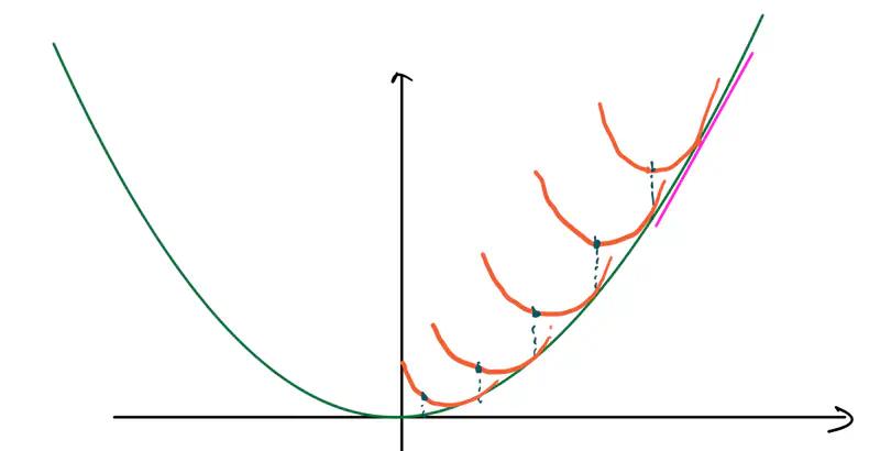
Draw a parabola at \(x_k\) that locally approximates the function.
Jump directly to the minimum of that parabola; that’s the next step. Note: So, instead of walking down the slope step by step (gradient descent), we are jumping straight to the point where the curve bends downwards towards the bottom.

\[ x_{k+1} = x_k - \frac{f\prime(x_k)}{f\prime\prime(x_k)} \\[10pt] \text{ step size = } \frac{1}{f\prime\prime(x_k)} \\[10pt] f\prime\prime(x_k) : \text{ tells curvature of the function at } x_k \\[10pt] x_{new} = x_{old} - (\nabla^2 f(x_{old})^{-1} \nabla f(x_{old}) \\[10pt] \nabla^2 f(x_{old}): Hessian \]

For example:

Find the minima of \(f(x) = x^2 - 4x + 5\) To find the minima, lets calulate the first derivative and equate to zero.
\(f'(x) = 2x - 4 = 0 \)
\( => x^* = 2 \)

\(f''(x) = 2 >0 \) => minima is at \(x^* = 2\)

Now, we will solve this using Newton’s Method.
Let’s start at x = 0.

\[ x_{new} = x_{old} - \frac{f\prime(x_{old})}{f\prime\prime(x_{old}} \\[10pt] => x_{new} = 0 - \frac{2*0 -4}{2} = 0-(-2) \\[10pt] => x_{new} = 2 \]

Hence, we can see that using Newton’s Method we can get to the minima \(x^* = 2\) in just 1 step.

Limitations

Full Newton’s Method is rarely used in Machine Learning/Deep Learning optimization, because of the following limitations:

\(TC = O(n^2\)) for Hessian calculation, since for a network with \(n\) parameters
requires \(n^2\) derivative calculations.
\(TC = O(n^3\)) for Hessian Inverse calculation.
If it encounters a Saddle point, then it can go to a maxima rather than minima.

Because of the above limitations, we use Quasi-Newton methods like BFGS and L-BFGS.
The quasi-Newton methods make use of approximations for Hessian calculation, in order to gain the benefits of curvature without incurring the cost of Hessian calculation.

BFGS: Broyden-Fletcher-Goldfarb-Shanno
L-BFGS: Limited-memory BFGS

Watch Video

End of Section