This is the multi-page printable view of this section. Click here to print.
Linear Algebra
1 - Vector Fundamentals
It is used to describe the surrounding space, e.g, lines, planes, 3D space, etc.
And, In machine learning, vectors are used to represent data, both the input features and the output of a model.
It is a collection of scalars(numbers) that has both magnitude and direction.
Geometrically, it is a line segment in space characterized by its length(magnitude) and direction.
By convention, we represent vectors as column vectors.
e.g.:
\(\vec{x} = \mathbf{x} = \begin{bmatrix} x_1 \\ x_2 \\ \vdots \\ x_n \end{bmatrix}_{\text{n×1}}\) i.e ’n’ rows and 1 column.
Important: In machine learning, we will use bold notation \(\mathbf{v}\) to represent vectors, instead
of arrow notation \(\mathbf{v}\).
Swap the rows and columns, i.e, a column vector becomes a row vector after transpose.
e.g:
\(\mathbf{v} = \begin{bmatrix} v_1 \\ v_2 \\ \vdots \\ v_d \end{bmatrix}_{\text{d×1}}\)
\(\mathbf{v}^\mathrm{T} = \begin{bmatrix} v_1 & v_2 & \cdots & v_d \end{bmatrix}_{\text{1×d}}\)
The length (or magnitude or norm) of a vector \(\mathbf{v}\) is the distance from the origin to the point represented
by \(\mathbf{v}\) in n-dimensional space.
\(\mathbf{v} = \begin{bmatrix} v_1 \\ v_2 \\ \vdots \\ v_d \end{bmatrix}_{\text{d×1}}\)
Length of vector:
Note: The length of a zero vector is 0.
The direction of a vector tells us where the vector points in space, independent of its length.
Direction of vector:
\[\mathbf{v} = \frac{\vec{v}} {\|\mathbf{v}\|} \]It is a collection of vectors that can be added together and scaled by numbers (scalars), such that,
the results are still in the same space.
Vector space or linear space is a non-empty set of vectors equipped with 2 operations:
- Vector addition: for any 2 vectors \(a, b\), \(a + b\) is also in the same vector space.
- Scalar multiplication: for a vector \(\mathbf{v}\), \(\alpha\mathbf{v}\) is also in the same vector space;
where \(\alpha\) is a scalar.
Note: These operations must satisfy certain rules (called axioms), such as, associativity, commutativity, distributivity, existence of a zero vector, and additive inverses.
e.g.: Set of all points in 2D is a vector space.
Addition:
We can only add vectors of the same dimension.
- Commutative: \(a + b = b + a\)
- Associative: \(a + (b + c) = (a + b) + c\)
e.g: lets add 2 real d-dimensional vectors, \(\mathbf{u} , \mathbf{v} \in \mathbb{R}^{d \times 1}\):
\(\mathbf{u} = \begin{bmatrix} u_1 \\ u_2 \\ \vdots \\ u_d \end{bmatrix}_{\text{d×1}}\),
\(\mathbf{v} = \begin{bmatrix} v_1 \\ v_2 \\ \vdots \\ v_d \end{bmatrix}_{\text{d×1}}\)
\(\mathbf{u} + \mathbf{v} = \begin{bmatrix} u_1+v_1 \\ u_2+v_2 \\ \vdots \\ u_d+v_d \end{bmatrix}_{\text{d×1}}\)
Multiplication:
1. Multiplication with Scalar:
All elements of the vector are multiplied with the scalar.
- \(c(\mathbf{u} + \mathbf{v}) = c(\mathbf{u}) + c(\mathbf{v})\)
- \((c+d)\mathbf{v} = c\mathbf{v} + d\mathbf{v}\)
- \((cd)\mathbf{v} = c(d\mathbf{v})\)
e.g:
\(\alpha\mathbf{v} = \begin{bmatrix} \alpha v_1 \\ \alpha v_2 \\ \vdots \\ \alpha v_d \end{bmatrix}_{\text{d×1}}\)
2.Inner (Dot) Product:
Inner(dot) product \(\mathbf{u} \cdot \mathbf{v}\) of 2 vectors gives a scalar output.
The two vectors must be of the same dimensions.
- \(\mathbf{u} \cdot \mathbf{v} = u_1v_1 + u_2v_2 + \cdots + u_dv_d\)
Dot product:
\(\mathbf{u} \cdot \mathbf{v} = \mathbf{u}^\mathrm{T} \mathbf{v}\)
= \(\begin{bmatrix} u_1 & u_2 & \cdots & u_d \end{bmatrix}_{\text{1×d}}
\cdot
\begin{bmatrix} v_1 \\ v_2 \\ \vdots \\ v_d
\end{bmatrix}_{\text{d×1}} = u_1v_1 + u_2v_2 + \cdots + u_dv_d\)
Geometrically, \(\mathbf{u} \cdot \mathbf{v}\) = \(|u||v|cos\theta\)
where \(\theta\) is the angle between \(\mathbf{u}\) and \(\mathbf{v}\).
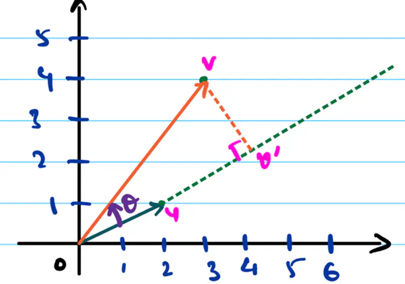
\(\mathbf{u} = \begin{bmatrix} 1 \\ \\ 2 \\ \end{bmatrix}_{\text{2×1}}\), \(\mathbf{v} = \begin{bmatrix} 3 \\ \\ 4 \\ \end{bmatrix}_{\text{2×1}}\)
\(\mathbf{u} \cdot \mathbf{v}\) = \(|u||v|cos\theta = 1 \times 3 + 2 \times 4 = 11\)
2.Outer (Tensor) Product:
Outer (tensor) product \(\mathbf{u} \otimes \mathbf{v}\) of 2 vectors gives a matrix output.
The two vectors must be of the same dimensions.
Tensor product:
\(\mathbf{u} \otimes \mathbf{v} = \mathbf{u} \mathbf{v}^\mathrm{T} \)
= \(\begin{bmatrix} u_1 \\ u_2 \\ \vdots \\ u_d \end{bmatrix}_{\text{d×1}}
\otimes
\begin{bmatrix} v_1 & v_2 & \cdots & v_d \end{bmatrix}_{\text{1×d}}
= \begin{bmatrix}
u_1v_1 & u_1v_2 & \cdots & u_1v_d \\
u_2v_1 & u_2v_2 & \cdots & u_2v_n \\
\vdots & \vdots & \ddots & \vdots \\
u_dv_1 & u_dv_2 & \cdots & u_dv_d
\end{bmatrix}
\in \mathbb{R}^{d \times d}\)
e.g:
\(\mathbf{u} = \begin{bmatrix} 1 \\ \\ 2 \\ \end{bmatrix}_{\text{2×1}}\),
\(\mathbf{v} = \begin{bmatrix} 3 \\ \\ 4 \\ \end{bmatrix}_{\text{2×1}}\)
\(\mathbf{u} \otimes \mathbf{v} = \mathbf{u} \mathbf{v}^\mathrm{T} \) = \(\begin{bmatrix} 1 \\ \\ 2 \\ \end{bmatrix}_{\text{2×1}} \otimes \begin{bmatrix} 3 & 4 \end{bmatrix}_{\text{1×2}} = \begin{bmatrix} 1 \times 3 & 1 \times 4 \\ \\ 2 \times 3 & 2 \times 4 \\ \end{bmatrix} _{\text{2×2}} = \begin{bmatrix} 3 & 4 \\ \\ 6 & 8 \\ \end{bmatrix} _{\text{2×2}}\)
Note: We will NOT discuss about cross product \(\mathbf{u} \times \mathbf{v}\); product perpendicular to both vectors.
\(\mathbf{v} = \alpha_1 \mathbf{u}_1 + \alpha_2 \mathbf{u}_2 + \cdots + \alpha_k \mathbf{u}_k\)
where \(\alpha_1, \alpha_2, \cdots, \alpha_k\) are scalars.
A set of vectors are linearly independent if NO vector in the set can be expressed as a linear combination of
the other vectors in the set.
The only solution for :
\(\alpha_1 \mathbf{u}_1 + \alpha_2 \mathbf{u}_2 + \cdots + \alpha_k \mathbf{u}_k\) = 0
is \(\alpha_1 = \alpha_2, \cdots, = \alpha_k = 0\).
e.g.:
The below 3 vectors are linearly independent.
\(\mathbf{u} = \begin{bmatrix} 1 \\ 1 \\ 1 \\ \end{bmatrix}_{\text{3×1}}\), \(\mathbf{v} = \begin{bmatrix} 1 \\ 2 \\ 3 \\ \end{bmatrix}_{\text{3×1}}\), \(\mathbf{w} = \begin{bmatrix} 1 \\ 3 \\ 6 \\ \end{bmatrix}_{\text{3×1}}\)The below 3 vectors are linearly dependent.
\(\mathbf{u} = \begin{bmatrix} 1 \\ 1 \\ 1 \\ \end{bmatrix}_{\text{3×1}}\), \(\mathbf{v} = \begin{bmatrix} 1 \\ 2 \\ 3 \\ \end{bmatrix}_{\text{3×1}}\), \(\mathbf{w} = \begin{bmatrix} 2 \\ 4 \\ 6 \\ \end{bmatrix}_{\text{3×1}}\)
because, \(\mathbf{w} = 2\mathbf{v}\), and we have a non-zero solution for the below equation:
\(\alpha_1 \mathbf{u} + \alpha_2 \mathbf{v} + \alpha_3 \mathbf{w} = 0\);
\(\alpha_1 = 0, \alpha_2 = -2, \alpha_3 = 1\) is a valid non-zero solution.
Note:
- A common method to check linear independence is to arrange the column vectors in a matrix form and calculate its determinant, if determinant ≠ 0, then the vectors are linearly independent.
- If number of vectors > number of dimensions, then the vectors are linearly dependent.
Since, the \((n+1)^{th}\) vector can be expressed as a linear combination of the other ’n’ vectors in n-dimensional space. - In machine learning, if a feature can be expressed in terms of other features, then it is linearly dependent,
and the feature is NOT bringing any new information.
e.g.: In 2 dimensions, 3 vectors \(\mathbf{x_1}, \mathbf{x_2}, \mathbf{x_3} \) are linearly dependent.
Span of a set of vectors is the geometric shape by all possible linear combinations of those vectors, such as,
line, plane, or higher dimensional volume.
e.g.:
- Span of a single vector (1,0) is the entire X-axis.
- Span of 2 vectors (1,0) and (0,1) is the entire X-Y (2D) plane, as any vector in 2D plane can be expressed as a linear combination of the 2 vectors - (1,0) and (0,1).
It is the minimal set of linearly independent vectors that spans or defines the entire vector space,
providing a unique co-ordinate system for every vector within the space.
Every vector in the vector space can be represented as a unique linear combination of the basis vectors.
e.g.:
- X-axis(1,0) and Y-axis(0,1) are the basis vectors of 2D space or form the co-ordinate system.
- \(\mathbf{u} = (3,1)\) and \(\mathbf{v} = (-1, 2) \) are the basis of skewed or parallelogram co-ordinate system.
Note: Basis = Dimensions
Two vectors are orthogonal if their dot product is 0.
A set of vectors \(\mathbf{x_1}, \mathbf{x_2}, \cdots ,\mathbf{x_n} \) are said to be orthogonal if:
\(\mathbf{x_i} \cdot \mathbf{x_j} = 0 \forall i⍯j\), for every pair, i.e, every pair must be orthogonal.
e.g.:
- \(\mathbf{u} = (1,0)\) and \(\mathbf{v} = (0,1) \) are orthogonal vectors.
- \(\mathbf{u} = (1,0)\) and \(\mathbf{v} = (1,1) \) are NOT orthogonal vectors.
Note:
Orthogonal vectors are linearly independent, but the inverse may NOT be true,
i.e, linear independence does NOT imply that vectors are orthogonal. e.g.:
Vectors \(\mathbf{u} = (2,0)\) and \(\mathbf{v} = (1,3) \) are linearly independent but NOT orthogonal.
Since, \(\mathbf{u} \cdot \mathbf{v} = 2*1 + 3*0 = 2 ⍯ 0\).Orthogonality is the most extreme case of linear independence, i.e \(90^{\degree}\) apart or perpendicular.
Orthonormal vectors are vectors that are orthogonal and have unit length.
A set of vectors \(\mathbf{x_1}, \mathbf{x_2}, \cdots ,\mathbf{x_n} \) are said to be orthonormal if:
\(\mathbf{x_i} \cdot \mathbf{x_j} = 0 \forall i⍯j\) and \(\|\mathbf{x_i}\| = 1\), i.e, unit vector.
e.g.:
- \(\mathbf{u} = (1,0)\) and \(\mathbf{v} = (0,1) \) are orthonormal vectors.
- \(\mathbf{u} = (1,0)\) and \(\mathbf{v} = (0,2) \) are NOT orthonormal vectors.
It is a set of vectors that functions as a basis for a space while also being orthonormal,
meaning each vector is a unit vector (has a length of 1) and all vectors are mutually perpendicular (orthogonal) to each other.
A set of vectors \(\mathbf{x_1}, \mathbf{x_2}, \cdots ,\mathbf{x_n} \) are said to be orthonormal basis of a vector space
\(\mathbb{R}^{n \times 1}\), if every vector:
e.g.:
- \(\mathbf{u} = (1,0)\) and \(\mathbf{v} = (0,1) \) form an orthonormal basis for 2-D space.
- \(\mathbf{u} = (\frac{1}{\sqrt{2}},\frac{1}{\sqrt{2}})\) and \(\mathbf{v} = (-\frac{1}{\sqrt{2}},-\frac{1}{\sqrt{2}}) \)
also form an orthonormal basis for 2-D space.
Note: In a n-dimensional space, there are only \(n\) possible orthonormal bases.
End of Section
2 - Matrix Operations
Matrices let us store, manipulate, and transform data efficiently.
e.g:
- Represent a system of linear equations AX=B.
- Data representation, such as images, that are stored as a matrix of pixels.
- When multiplied, matrix, linearly transforms a vector, i.e, its direction and magnitude, making it useful in image rotation, scaling, etc.
e.g:
\( \mathbf{A} = \begin{bmatrix} a_{11} & a_{12} & \cdots & a_{1n} \\ a_{21} & a_{22} & \cdots & a_{2n} \\ \vdots & \vdots & \ddots & \vdots \\ a_{m1} & a_{m2} & \cdots & a_{mn} \end{bmatrix} _{\text{m x n}} \)
\( \mathbf{A}^T = \begin{bmatrix} a_{11} & a_{21} & \cdots & a_{m1} \\ a_{12} & a_{22} & \cdots & a_{m2} \\ \vdots & \vdots & \ddots & \vdots \\ a_{1n} & a_{2n} & \cdots & a_{mn} \end{bmatrix} _{\text{n x m}} \)
Important: \( (AB)^T = B^TA^T \)
Addition:
We add two matrices by adding the corresponding elements.
They must have same dimensions.
\( \mathbf{A} + \mathbf{B} =
\begin{bmatrix}
a_{11} + b_{11} & a_{12} + b_{12} & \cdots & a_{1n} + b_{1n} \\
a_{21} + b_{21} & a_{22} + b_{22} & \cdots & a_{2n} + b_{2n} \\
\vdots & \vdots & \ddots & \vdots \\
a_{m1} + b_{m1} & a_{m2} + b_{m2} & \cdots & a_{mn} + b_{mn}
\end{bmatrix}
_{\text{m x n}}
\)
Multiplication:
We can multiply two matrices only if their inner dimensions are equal.
\( \mathbf{C}_{m x n} = \mathbf{A}_{m x d} ~ \mathbf{B}_{d x n} \)
\( c_{ij} \) = Dot product of \(i^{th}\) row of A and \(j^{th}\) row of B.
\( c_{ij} = \sum_{k=1}^{d} A_{ik} * B_{kj} \)
=> \( c_{11} = a_{11} * b_{11} + a_{12} * b_{21} + \cdots + a_{1d} * b_{d1} \)
e.g:
\(
\mathbf{A} =
\begin{bmatrix}
1 & 2 \\
\\
3 & 4
\end{bmatrix}
_{\text{2 x 2}},
\mathbf{B} =
\begin{bmatrix}
5 & 6 \\
\\
7 & 8
\end{bmatrix}
_{\text{2 x 2}}
\)
\(
\mathbf{C} = \mathbf{A} \times \mathbf{B} =
\begin{bmatrix}
1 * 5 + 2 * 7 & 1 * 6 + 2 * 8 \\
\\
3 * 5 + 4 * 7 & 3 * 6 + 4 * 8
\end{bmatrix}
_{\text{2 x 2}}
= \begin{bmatrix}
19 & 22 \\
\\
43 & 50
\end{bmatrix}
_{\text{2 x 2}}
\)
Key Properties:
- AB ≠ BA ; NOT commutative
- (AB)C = A(BC) ; Associative
- A(B+C) = AB+AC ; Distributive
Square Matrix:
It is a matrix with same number of rows and columns (m=n).
\(
\mathbf{A} =
\begin{bmatrix}
a_{11} & a_{12} & \cdots & a_{1n} \\
a_{21} & a_{22} & \cdots & a_{2n} \\
\vdots & \vdots & \ddots & \vdots \\
a_{n1} & a_{n2} & \cdots & a_{nn}
\end{bmatrix}
_{\text{n x n}}
\)
Diagonal Matrix:
It is a square matrix with all non-diagonal elements equal to zero.
e.g.:
\( \mathbf{D} =
\begin{bmatrix}
d_{11} & 0 & \cdots & 0 \\
0 & d_{22} & \cdots & 0 \\
\vdots & \vdots & \ddots & \vdots \\
0 & 0 & \cdots & d_{nn}
\end{bmatrix}
_{\text{n x n}}
\)
Note: Product of 2 diagonal matrices is a diagonal matrix.
Lower Triangular Matrix:
It is a square matrix with all elements above the diagonal equal to zero.
e.g.:
\( \mathbf{L} =
\begin{bmatrix}
l_{11} & 0 & \cdots & 0 \\
l_{21} & l_{22} & \cdots & 0 \\
\vdots & \vdots & \ddots & \vdots \\
l_{n1} & l_{n2} & \cdots & l_{nn}
\end{bmatrix}
_{\text{n x n}}
\)
Note: Product of 2 lower triangular matrices is an lower triangular matrix.
Upper Triangular Matrix:
It is a square matrix with all elements below the diagonal equal to zero.
e.g.:
\( \mathbf{U} =
\begin{bmatrix}
u_{11} & u_{12} & \cdots & u_{1n} \\
0 & u_{22} & \cdots & u_{2n} \\
\vdots & \vdots & \ddots & \vdots \\
0 & 0 & \cdots & u_{nn}
\end{bmatrix}
_{\text{n x n}}
\)
Note: Product of 2 upper triangular matrices is an upper triangular matrix.
Symmetric Matrix:
It is a square matrix that is equal to its own transpose, i.e, flip the matrix along its diagonal,
it remains unchanged.
\( \mathbf{A} = \mathbf{A}^T \)
e.g.:
\( \mathbf{S} =
\begin{bmatrix}
s_{11} & s_{12} & \cdots & s_{1n} \\
s_{12} & s_{22} & \cdots & s_{2n} \\
\vdots & \vdots & \ddots & \vdots \\
s_{1n} & s_{2n} & \cdots & s_{nn}
\end{bmatrix}
_{\text{n x n}}
\)
Note: Diagonal matrix is a symmetric matrix.
Skew Symmetric Matrix:
It is a square symmetric matrix where the elements across the diagonal have opposite signs.
Also called Anti Symmetric Matrix.
\( \mathbf{A} = -\mathbf{A}^T \)
e.g.:
\( \mathbf{S} =
\begin{bmatrix}
0 & s_{12} & \cdots & s_{1n} \\
-s_{12} & 0 & \cdots & s_{2n} \\
\vdots & \vdots & \ddots & \vdots \\
-s_{1n} & -s_{2n} & \cdots & 0
\end{bmatrix}
_{\text{n x n}}
\)
Note: Diagonal elements of a skew symmetric matrix are zero, since the number should be equal to its negative.
Identity Matrix:
It is a square matrix with all the diagonal values equal to 1, rest of the elements are equal to zero.
e.g.:
\( \mathbf{I} =
\begin{bmatrix}
1 & 0 & \cdots & 0 \\
0 & 1 & \cdots & 0 \\
\vdots & \vdots & \ddots & \vdots \\
0 & 0 & \cdots & 1
\end{bmatrix}
_{\text{n x n}}
\)
Important:
\( \mathbf{I} \times \mathbf{A} = \mathbf{A} \times \mathbf{I} = \mathbf{A} \)
Trace:
It is the sum of the elements on the main diagonal of a square matrix.
Note: Main diagonal is NOT defined for a rectangular matrix.
\( \text{trace}(A) = \sum_{i=1}^{n} a_{ii} = a_{11} + a_{22} + \cdots + a_{nn}\)
If \( \mathbf{A} \in \mathbb{R}^{m \times n} \), and \( \mathbf{B} \in \mathbb{R}^{n \times m} \), then
\( \text{trace}(AB)_{m \times m} = \text{trace}(BA)_{n \times n} \)
Determinant:
It is a scalar value that reveals crucial properties about the matrix and its linear transformation.
- If determinant = 0 => singular matrix, i.e linearly dependent rows or columns.
- Determinant is also equal to the scaling factor of the linear transformation.
\(a_{1j} \) = element in the first row and j-th column
\(M_{1j} \) = submatrix of the matrix excluding the first row and j-th column
If n = 2, then,
\( |A| = a_{11} \, a_{22} - a_{12} \, a_{21} \)
Singular Matrix:
A square matrix with linearly dependent rows or columns, i.e, determinant = 0.
A singular matrix collapses space, say, a 3D space, into a 2D space or a higher dimensional space
to a lower dimensional space, making the transformation impossible to reverse.
Hence, a singular matrix is NOT invertible; i.e, inverse does NOT exist.
Singular matrix is also NOT invertible, because the inverse has division by determinant, and its determinant is zero.
Also called rank deficient matrix, because the rank < number of dimensions of the matrix,
due to the presence of linearly dependent rows or columns.
e.g: Below is a linearly dependent 2x2 matrix.
\( \mathbf{A} =
\begin{bmatrix}
a_{11} & a_{12} \\
\\
\beta a_{11} & \beta a_{12}
\end{bmatrix}
_{\text{2 x 2}},
det(\mathbf{A}) =
a_{11}\cdot \beta a_{12} - a_{12} \cdot \beta a_{11} = 0
\)
Note:
- \( det(A) = det(A^T) \)
- \( det(\beta A) = \beta^n det(A) \), where n is the number of dimensions of A and \(\beta\) is a scalar.
Inverse:
It is a square matrix that when multiplied by the original matrix, gives the identity matrix.
\( \mathbf{A} \mathbf{A}^{-1} = \mathbf{A}^{-1} \mathbf{A} = \mathbf{I} \)
Steps to compute inverse of a matrix:
- Calculate the determinant of the matrix. \( |A| = \det(A) \)
- For each element \(a_{ij}\), compute its minor \(M_{ij}\).
\(M_{ij}\) is the determinant of the submatrix of the matrix excluding the i-th row and j-th column. - Form the co-factor matrix \(C_{ij}\), using the minor.
\( C_{ij} = (-1)^{\,i+j}\,M_{ij} \) - Take the transpose of the cofactor matrix to get the adjugate matrix.
\( \mathrm{adj}(A) = \mathrm{C}^\mathrm{T} \) - Compute the inverse:
\( A^{-1} = \frac{1}{|A|}\,\mathrm{adj}(A) = \frac{1}{|A|}\,\mathrm{C}^\mathrm{T}\)
e.g:
\(
\mathbf{A} =
\begin{bmatrix}
1 & 0 & 3\\
2 & 1 & 1\\
1 & 1 & 1 \\
\end{bmatrix}
_{\text{3 x 3}}
\),
Co-factor matrix:
\(
\mathbf{C} =
\begin{bmatrix}
0 & -1 & 1\\
3 & -2 & -1\\
-3 & 5 & 1 \\
\end{bmatrix}
_{\text{3 x 3}}
\)
Adjugate matrix, adj(A) =
\(
\mathbf{C}^\mathrm{T} =
\begin{bmatrix}
0 & 3 & -3\\
-1 & -2 & 5\\
1 & -1 & 1 \\
\end{bmatrix}
_{\text{3 x 3}}
\)
determinant of \( \mathbf{A} \) =
\(
\begin{vmatrix}
1 & 0 & 3\\
2 & 1 & 1\\
1 & 1 & 1 \\
\end{vmatrix}
= 0 -\cancel 1 + \cancel 1 + \cancel3 - 2 -\cancel1 -\cancel 3 + 5 + \cancel1 = 3
\)
\(
\mathbf{A}^{-1} = \frac{1}{|A|}\,\mathrm{adj}(A)
= \frac{1}{3}\,
\begin{bmatrix}
0 & 3 & -3\\
-1 & -2 & 5\\
1 & -1 & 1 \\
\end{bmatrix}
_{\text{3 x 3}}
\)
=> \(
\mathbf{A}^{-1} =
\begin{bmatrix}
0 & 1 & -1\\
-1/3 & -2/3 & 5/3\\
1/3 & -1/3 & 1/3 \\
\end{bmatrix}
_{\text{3 x 3}}
\)
Note:
- Inverse of an Identity matrix is the Identity matrix itself.
- Inverse of \( \beta \mathbf{A} = \frac{1}{\beta}\mathbf{A}^{-1} \).
- \( (\mathbf{A}^\mathrm{T})^{-1} = (\mathbf{A}^{-1})^\mathrm{T} \).
- Inverse of a diagonal matrix is a diagonal matrix with reciprocal of the diagonal elements.
- Inverse of a upper triangular matrix is the upper triangular matrix.
- Inverse of a lower triangular matrix is the lower triangular matrix.
- Symmetric matrix, if invertible, then \((\mathbf{A}^{-1})^\mathrm{T} = \mathbf{A}^{-1}\), since, \(\mathbf{A} = \mathbf{A}^\mathrm{T}\)
It is a square matrix that whose rows and columns are orthonormal vectors, i.e, they are perpendicular to each other
and have a unit length.
\( \mathbf{A} \mathbf{A}^\mathrm{T} = \mathbf{A}^\mathrm{T} \mathbf{A} = \mathbf{A} \mathbf{A}^{-1} = \mathbf{I} \)
=> \( \mathbf{A}^\mathrm{T} = \mathbf{A}^{-1} \)
Note:
- Orthogonal matrix preserves the length and angles of vectors, acting as rotation or reflection in geometry.
- The determinant of an orthogonal matrix is always +1 or -1, because \( \mathbf{A} \mathbf{A}^\mathrm{T} = \mathbf{I} \)
Let’s check out why the rows and columns of an orthogonal matrix are orthonormal.
\( \mathbf{A} =
\begin{bmatrix}
a_{11} & a_{12} \\
\\
a_{21} & a_{22}
\end{bmatrix}
_{\text{2 x 2}}
\),
=> \( \mathbf{A}^\mathrm{T} =
\begin{bmatrix}
a_{11} & a_{21} \\
\\
a_{12} & a_{22}
\end{bmatrix}
_{\text{2 x 2}}
\)
Since, \( \mathbf{A} \mathbf{A}^\mathrm{T} = \mathbf{I} \)
\(
\begin{bmatrix}
a_{11} & a_{12} \\
\\
a_{21} & a_{22}
\end{bmatrix}
\begin{bmatrix}
a_{11} & a_{21} \\
\\
a_{12} & a_{22}
\end{bmatrix}
= \begin{bmatrix}
a_{11}^2 + a_{12}^2 & a_{11}a_{21} + a_{12}a_{22} \\
\\
a_{21}a_{11} + a_{21}a_{12} & a_{21}^2 + a_{22}^2
\end{bmatrix}
= \begin{bmatrix}
1 & 0 \\
\\
0 & 1
\end{bmatrix}
\)
Equating the terms, we get:
\( a_{11}^2 + a_{12}^2 = 1 \) => row 1 is a unit vector
\( a_{21}^2 + a_{22}^2 = 1 \) => row 2 is a unit vector
\( a_{11}a_{21} + a_{12}a_{22} = 0 \) => row 1 and row 2 are orthogonal to each other, since dot product = 0
\( a_{21}a_{11} + a_{21}a_{12} = 0 \) => row 1 and row 2 are orthogonal to each other, since dot product = 0
Therefore, the rows and columns of an orthogonal matrix are orthonormal.
Let, \(\mathbf{Q}\) is an orthogonal matrix, and \(\mathbf{v}\) is a vector.
Let’s calculate the length of \( \mathbf{Q} \mathbf{v} \)
Therefore, linear transformation of a vector by an orthogonal matrix does NOT change its length.
\( 2x + y = 5 \)
\( x + 2y = 4 \)
Lets solve the system of equations using matrix:
\(\begin{bmatrix}
2 & 1 \\
\\
1 & 2
\end{bmatrix}
\)
\(
\begin{bmatrix}
x \\
\\
y
\end{bmatrix}
= \begin{bmatrix}
5 \\
\\
4
\end{bmatrix}
\)
The above equation can be written as:
\(\mathbf{AX} = \mathbf{B} \)
=> \( \mathbf{X} = \mathbf{A}^{-1} \mathbf{B} \)
\( \mathbf{A} = \begin{bmatrix}
2 & 1 \\
\\
1 & 2
\end{bmatrix},
\mathbf{B} = \begin{bmatrix}
5 \\
\\
4
\end{bmatrix},
\mathbf{X} = \begin{bmatrix}
x \\
\\
y
\end{bmatrix}
\)
Lets compute the inverse of A matrix:
\( \mathbf{A}^{-1} = \frac{1}{3}\begin{bmatrix}
2 & -1 \\
\\
-1 & 2
\end{bmatrix}
\)
Since, \( \mathbf{X} = \mathbf{A}^{-1} \mathbf{B} \)
=> \( \mathbf{X} = \begin{bmatrix}
x \\
\\
y
\end{bmatrix}
= \frac{1}{3}\begin{bmatrix}
2 & -1 \\
\\
-1 & 2
\end{bmatrix}
\begin{bmatrix}
5 \\
\\
4
\end{bmatrix}
= \frac{1}{3}\begin{bmatrix}
6 \\
\\
3
\end{bmatrix}
= = \begin{bmatrix}
2 \\
\\
1
\end{bmatrix}
\)
Therefore, \( x = 2 \) and \( y = 1 \).
End of Section
3 - Eigen Value Decomposition
It tells us about the characteristic properties of a matrix.
Multiplying a vector by a matrix can change the direction or magnitude or both of the vector.
\( \mathbf{A} = \begin{bmatrix}
2 & 1 \\
\\
1 & 2
\end{bmatrix}
\),
\(\mathbf{u} = \begin{bmatrix} 0 \\ \\ 1 \\ \end{bmatrix}\),
\(\mathbf{v} = \begin{bmatrix} 1 \\ \\ 1 \\ \end{bmatrix}\)
\(\mathbf{Au} = \begin{bmatrix} 1 \\ \\ 2 \\ \end{bmatrix}\) , \(\quad\)
\(\mathbf{Av} = \begin{bmatrix} 3 \\ \\ 3 \\ \end{bmatrix}\)
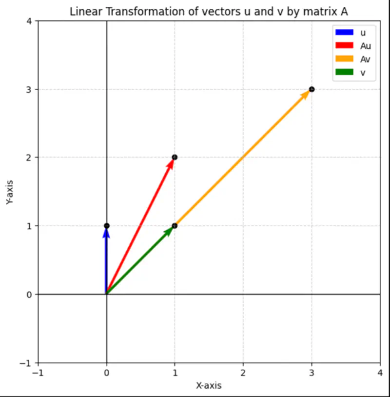
It might get scaled up or down but does not change its direction.
Result of linear transformation, i.e, multiplying the vector by a matrix, is just a scalar multiple of the original vector.
\(|\lambda| > 1 \): Vector stretched
\(0 < |\lambda| < 1 \): Vector shrunk
\(|\lambda| = 1 \): Same size
\(\lambda < 0 \): Vector’s direction is reversed
Since, for an eigen vector, result of linear transformation, i.e, multiplying the vector by a matrix, is just a scalar multiple of the original vector, =>
\[ \mathbf{A} \mathbf{v} = \lambda \mathbf{v} \\ \mathbf{A} \mathbf{v} - \lambda \mathbf{v} = 0 \\ \mathbf{v}(\mathbf{A} - \lambda \mathbf{I}) = 0 \\ \]For a non-zero eigen vector, \((\mathbf{A} - \lambda \mathbf{I})\) must be singular, i.e,
\(det(\mathbf{A} - \lambda \mathbf{I}) = 0 \)
If, \( \mathbf{A} =
\begin{bmatrix}
a_{11} & a_{12} & \cdots & a_{1n} \\
a_{21} & a_{22} & \cdots & a_{2n} \\
\vdots & \vdots & \ddots & \vdots \\
a_{n1} & a_{n2} & \cdots & a_{nn}
\end{bmatrix}
_{\text{n x n}}
\),
then, \((\mathbf{A} - \lambda \mathbf{I}) =
\begin{bmatrix}
a_{11}-\lambda & a_{12} & \cdots & a_{1n} \\
a_{21} & a_{22}-\lambda & \cdots & a_{2n} \\
\vdots & \vdots & \ddots & \vdots \\
a_{n1} & a_{n2} & \cdots & a_{nn}-\lambda
\end{bmatrix}
_{\text{n x n}}
\)
\(det(\mathbf{A} - \lambda \mathbf{I})) = 0 \), will give us a polynomial equation in \(\lambda\) of degree \(n\),
we need to solve this polynomial equation to get the \(n\) eigen values.
e.g.:
\( \mathbf{A} = \begin{bmatrix}
2 & 1 \\
\\
1 & 2
\end{bmatrix}
\),
\( \quad det(\mathbf{A} - \lambda \mathbf{I})) = 0 \quad \) =>
\( det \begin{bmatrix}
2-\lambda & 1 \\
\\
1 & 2-\lambda
\end{bmatrix} = 0
\)
\( (2-\lambda)^2 - 1 = 0\)
\( => |\lambda - 2| = \pm 1 \)
\( => \lambda_1 = 3\) and \( \lambda_2 = 1\)
Therefore, eigen vectors corresponding to eigen values \(\lambda_1 = 3\) and \( \lambda_2 = 1\) are:
\((\mathbf{A} - \lambda \mathbf{I}) \mathbf{v} = 0 \)
\(\lambda_1 = 3\)
=>
\(
\begin{bmatrix}
2-3 & 1 \\
\\
1 & 2-3
\end{bmatrix} \begin{bmatrix} v_1 \\ \\ v_2 \\ \end{bmatrix} =
\begin{bmatrix}
-1 & 1 \\
\\
1 & -1
\end{bmatrix} \begin{bmatrix} v_1 \\ \\ v_2 \\ \end{bmatrix} = 0
\)
=> Both the equations will be \(v_1 - v_2 = 0 \), i.e, \(v_1 = v_2\)
So, we can choose any vector, where x-axis and y-axis components are same, i.e, \(v_1 = v_2\)
=> Eigen vector: \(v_1 = \begin{bmatrix} 1 \\ \\ 1 \\ \end{bmatrix}\)
Similarly, for \(\lambda_2 = 1\)
we will get, eigen vector: \(v_2 = \begin{bmatrix} 1 \\ \\ -1 \\ \end{bmatrix}\)
\(\mathbf{Iv} = \lambda \mathbf{v}\)
Therefore, identity matrix has only one eigen value \(\lambda = 1\), and all non-zero vectors can be eigen vectors.
\(\mathbf{A} = \begin{bmatrix} 0 & 1 \\ \\ -1 & 0 \end{bmatrix} \), \( \quad det(\mathbf{A} - \lambda \mathbf{I}) = 0 \quad \) => det \(\begin{bmatrix} 0-\lambda & 1 \\ \\ -1 & 0-\lambda \end{bmatrix} = 0 \)
=> \(\lambda^2 + 1 = 0\) => \(\lambda = \pm i\)
So, eigen values are complex.
e.g.:
\( \mathbf{D} = \begin{bmatrix} d_{11} & 0 & \cdots & 0 \\ 0 & d_{22} & \cdots & 0 \\ \vdots & \vdots & \ddots & \vdots \\ 0 & 0 & \cdots & d_{nn} \end{bmatrix} _{\text{n x n}} \), \( \quad det(\mathbf{D} - \lambda \mathbf{I}) = 0 \quad \) => det \( \begin{bmatrix} d_{11}-\lambda & 0 & \cdots & 0 \\ 0 & d_{22}-\lambda & \cdots & 0 \\ \vdots & \vdots & \ddots & \vdots \\ 0 & 0 & \cdots & d_{nn}-\lambda \end{bmatrix} _{\text{n x n}} \)
=> \((d_{11}-\lambda)(d_{22}-\lambda) \cdots (d_{nn}-\lambda) = 0\)
=> \(\lambda = d_{11}, d_{22}, \cdots, d_{nn}\)
So, eigen values are the diagonal elements of the matrix.
- For a \(n \times n\) matrix, there are \(n\) eigen values.
- Eigen values need NOT be unique, e.g, identity matrix has only one eigen value \(\lambda = 1\).
- Sum of eigen values = trace of matrix = sum of diagonal elements, i.e,
\(tr(\mathbf{A}) = \lambda_1 + \lambda_2 + \cdots + \lambda_n\). - Product of eigen values = determinant of matrix, i.e,
\(det(\mathbf{A}) = |\mathbf{A}|= \lambda_1 \lambda_2 \cdots \lambda_n\). e.g: For the example matrix given above,
\( \mathbf{A} = \begin{bmatrix} 2 & 1 \\ \\ 1 & 2 \end{bmatrix} \), \(\quad \lambda_1 = 3\) and \( \lambda_2 = 1\)
\(tr(\mathbf{A}) = 2 + 2 = 3 + 1 = 4\)
\(det(\mathbf{A}) = 2 \times 2 - 1 \times 1 = 3 \times 1 = 3 \)
- Eigen vectors corresponding to distinct eigen values of a real symmetric matrix are orthogonal to each other.
Proof:
Let, \(\mathbf{v_1}, \mathbf{v_2}\) be eigen vectors corresponding to distinct eigen value \(\lambda_1,\lambda_2\) of a real symmetric matrix \(\mathbf{A} = \mathbf{A}^T\).
We know that for eigen vectors -
\[ \mathbf{Av_1} = \lambda_1 \mathbf{v_1} ~and~ \mathbf{Av_2} = \lambda_2 \mathbf{v_2} \\[10pt] \text{ let's calculate the dot product: } \\[10pt] \mathbf{Av_1} \cdot \mathbf{v_2} = (\mathbf{Av_1})^T\mathbf{v_2} = \mathbf{v_1^TA^Tv_2} = \mathbf{v_1^T} ~ \mathbf{Av_2}, \quad \text {since } \mathbf{A} = \mathbf{A}^T\\[10pt] => (\mathbf{Av_1}) \cdot \mathbf{v_2} = \mathbf{v_1} \cdot (\mathbf{Av_2}) \\[10pt] => (\lambda_1 \mathbf{v_1}) \cdot \mathbf{v_2} = \mathbf{v_1} \cdot (\lambda_2\mathbf{v_2}) \\[10pt] => \lambda_1 (\mathbf{v_1 \cdot v_2}) = \lambda_2 (\mathbf{v_1 \cdot v_2}) \\[10pt] => (\lambda_1 - \lambda_2) (\mathbf{v_1} \cdot \mathbf{v_2}) = 0 \\[10pt] \text{ since, eigen values are distinct,} => \lambda_1 ≠ \lambda_2 \\[10pt] \therefore \mathbf{v_1} \cdot \mathbf{v_2} = 0 \\[10pt] => \text{ eigen vectors are orthogonal to each other,} => \mathbf{v_1} \perp \mathbf{v_2} \\[10pt] \]
Let’ calculate the 2nd power of a square matrix.
e.g.:
\(\mathbf{A} = \begin{bmatrix}
2 & 1 \\
\\
1 & 2
\end{bmatrix}
\),
\(\quad \mathbf{A}^2 = \begin{bmatrix}
2 & 1 \\
\\
1 & 2
\end{bmatrix} \begin{bmatrix}
2 & 1 \\
\\
1 & 2
\end{bmatrix} = \begin{bmatrix}
5 & 4 \\
\\
4 & 5
\end{bmatrix}
\)
So, we need to find an easier way to calculate the power of a matrix.
Let’s calculate the 2nd power of a diagonal matrix.
e.g.:
\(\mathbf{A} = \begin{bmatrix}
3 & 0 \\
\\
0 & 2
\end{bmatrix}
\),
\(\quad \mathbf{A}^2 = \begin{bmatrix}
3 & 0 \\
\\
0 & 2
\end{bmatrix} \begin{bmatrix}
3 & 0 \\
\\
0 & 2
\end{bmatrix} = \begin{bmatrix}
9 & 0 \\
\\
0 & 4
\end{bmatrix}
\)
Note that when we square the diagonal matrix, then all the diagonal elements got squared.
Similarly, if we want to calculate the kth power of a diagonal matrix, then all we need to do is to just compute the kth
powers of all diagonal elements, instead of complex matrix multiplications.
\(\quad \mathbf{A}^k = \begin{bmatrix}
3^k & 0 \\
\\
0 & 2^k
\end{bmatrix}
\)
Therefore, if we diagonalize a square matrix then the computation of power of the matrix will become very easy.
Next, let’s see how to diagonalize a matrix.
\(\mathbf{V}\): Matrix of all eigen vectors(as columns) of matrix \(\mathbf{A}\)
\( \mathbf{V} = \begin{bmatrix}
\mathbf{v}_1 & \mathbf{v}_2 & \cdots & \mathbf{v}_n \\
\vdots & \vdots & \ddots & \vdots \\
\vdots & \vdots & \vdots & \vdots\\
\end{bmatrix}
\),
where, each column is an eigen vector corresponding to an eigen value \(\lambda_i\).
If \( \mathbf{v}_1 \mathbf{v}_2 \cdots \mathbf{v}_n \) are linearly independent, then,
\(det(\mathbf{V}) ~⍯ ~ 0\).
=> \(\mathbf{V}\) is NOT singular and \(\mathbf{V}^{-1}\) exists.
\(\Lambda\): Diagonal matrix of all eigen values of matrix \(\mathbf{A}\)
\( \Lambda = \begin{bmatrix}
\lambda_1 & 0 & \cdots & 0 \\
\\
0 & \lambda_2 & \cdots & 0 \\
\vdots & \vdots & \ddots & \vdots \\
0 & 0 & \cdots & \lambda_n
\end{bmatrix}
\),
where, each diagonal element is an eigen value corresponding to an eigen vector \(\mathbf{v}_i\).
Let’s recall the characteristic equation of a matrix for calculating eigen values:
\(\mathbf{A} \mathbf{v} = \lambda \mathbf{v}\)
Let’s use the consolidated matrix for eigen values and eigen vectors described above:
i.e, \(\mathbf{A} \mathbf{V} = \mathbf{\Lambda} \mathbf{V}\)
For diagonalisation:
=> \(\mathbf{\Lambda} = \mathbf{V}^{-1} \mathbf{A} \mathbf{V}\)
We can see that, using the above equation, we can represent the matrix \(\mathbf{A}\) as a
diagonal matrix \(\mathbf{\Lambda}\) using the matrix of eigen vectors \(\mathbf{V}\).
Just reshuffling the above equation will give us the Eigen Value Decomposition of the matrix \(\mathbf{A}\):
\(\mathbf{A} = \mathbf{V} \mathbf{\Lambda} \mathbf{V}^{-1}\)
Important: Given that \(\mathbf{V}^{-1}\) exists, i.e, all the eigen vectors are linearly independent.
Let’s revisit the example given above:
\(\mathbf{A} = \begin{bmatrix}
2 & 1 \\
\\
1 & 2
\end{bmatrix}
\),
\(\quad \lambda_1 = 3\) and \( \lambda_2 = 1\),
\(\mathbf{v_1} = \begin{bmatrix} 1 \\ \\ 1 \\ \end{bmatrix}\),
\(\mathbf{v_2} = \begin{bmatrix} 1 \\ \\ -1 \\ \end{bmatrix}\)
=> \( \mathbf{V} = \begin{bmatrix}
1 & 1 \\
\\
1 & -1 \\
\end{bmatrix}
\),
\(\quad \mathbf{\Lambda} = \begin{bmatrix}
3 & 0 \\
\\
0 & 1
\end{bmatrix}
\)
\( \because \mathbf{A} = \mathbf{V} \mathbf{\Lambda} \mathbf{V}^{-1}\)
We know, \( \mathbf{V} ~and~ \mathbf{\Lambda} \), we need to calculate \(\mathbf{V}^{-1}\).
\(\mathbf{V}^{-1} = \frac{1}{2}\begin{bmatrix} 1 & 1 \\ \\ 1 & -1 \\ \end{bmatrix} \)
\( \therefore \mathbf{V} \mathbf{\Lambda} \mathbf{V}^{-1} = \begin{bmatrix}
1 & 1 \\
\\
1 & -1 \\
\end{bmatrix} \begin{bmatrix}
3 & 0 \\
\\
0 & 1
\end{bmatrix} \frac{1}{2}\begin{bmatrix}
1 & 1 \\
\\
1 & -1 \\
\end{bmatrix}
\)
\( = \frac{1}{2}
\begin{bmatrix}
3 & 1 \\
\\
3 & -1 \\
\end{bmatrix} \begin{bmatrix}
1 & 1 \\
\\
1 & -1 \\
\end{bmatrix} = \frac{1}{2}\begin{bmatrix}
4 & 2 \\
\\
2 & 4 \\
\end{bmatrix}
\)
\( = \begin{bmatrix}
2 & 1 \\
\\
1 & 2
\end{bmatrix} = \mathbf{A}
\)
Spectral decomposition is a specific type of eigendecomposition that applies to a symmetric matrix,
requiring its eigenvectors to be orthogonal.
In contrast, a general eigendecomposition applies to any diagonalizable matrix and does not require the eigenvectors
to be orthogonal.
The eigen vectors corresponding to distinct eigen values are orthogonal.
However, the matrix \(\mathbf{V}\) formed by the eigen vectors as columns is NOT orthogonal,
because the rows/columns are NOT orthonormal i.e unit length.
So, in order to make the matrix \(\mathbf{V}\) orthogonal, we need to normalize the rows/columns of the matrix
\(\mathbf{V}\), i.e, make, each eigen vector(column) unit length, by dividing the vector by its magnitude.
After normalisation we get orthogonal matrix \(\mathbf{Q}\) that is composed of unit length and orthogonal eigen vectors
or orthonormal eigen vectors.
Since, matrix \(\mathbf{Q}\) is orthogonal, => \(\mathbf{Q}^T = \mathbf{Q}^{-1}\)
The eigen value decomposition of a square matrix is:
\(\mathbf{A} = \mathbf{V} \mathbf{\Lambda} \mathbf{V}^{-1}\)
And, the spectral decomposition of a real symmetric matrix is:
\(\mathbf{A} = \mathbf{Q} \mathbf{\Lambda} \mathbf{Q}^T\)
Important: Note that, we are discussing only the special case of real symmetric matrix here,
because a real symmetric matrix is guaranteed to have all real eigenvalues.
- Principal Component Analysis (PCA): For dimensionality reduction.
- Page Rank Algorithm: For finding the importance of a web page.
- Structural Engineering: By calculating the eigen values of a bridge’s structural model, we can identify its natural frequencies to ensure that the bridge won’t resonate and be damaged by external forces, such as wind, and seismic waves.
End of Section
4 - Principal Component Analysis
In the diagram below, if we need to reduce the dimensionality of the data to 1, which feature should be dropped?
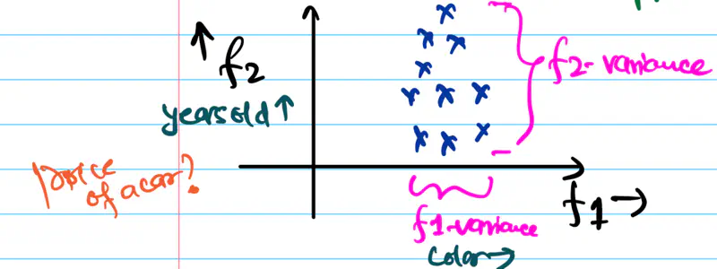
Since, information = variance, we should drop the feature that brings least information, i.e, has least variance.
Therefore, drop the feature 1.
What if the variance in both directions is same ?
What should be done in this case? Check the diagram below.
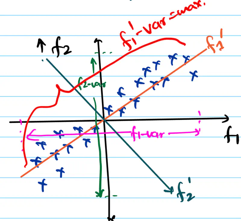
we will rotate the f1-axis in the direction of maximum spread/variance of data, i.e, f1’-axis and then we can drop f2’-axis, which is perpendicular to f1’-axis.
It is a dimensionality reduction technique that finds the direction of maximum variance in the data.
Note: Some loss of information will always be there in dimensionality reduction, because there will be some variability
in data along the direction that is dropped, and that will be lost.
Goal:
Fundamental goal of PCA is to find the new set of orthogonal axes, called the principal components, onto which
the data can be projected, such that, the variance of the projected data is maximum.
Say, we have data, \(D:X \in \mathbb{R}^{n \times d}\),
n is the number of samples
d is the number of features or dimensions of each data point.
In order to find the directions of maximum variance in data, we will use the covariance matrix of data.
Covariance matrix (C) summarizes the spread and relationship of the data in the original d-dimensional space.
\(C_{d \times d} = \frac{1}{n-1}X^TX \), where \(X\) is the data matrix.
Note: (n-1) in the denominator is for unbiased estimation(Bessel’s correction) of covariance matrix.
\(C_{ii}\) is the variance of the \(i^{th}\) feature.
\(C_{ij}\) is the co-variance between feature \(i\) and feature \(j\).
Trace(C) = Sum of diagonal elements of C = Total variance of data.
Algorithm:
Data is first mean centered, i.e, make mean = 0, i.e, subtract mean from each data point.
\(X = X - \mu\)Compute the covariance matrix with mean centered data.
\(C = \frac{1}{n-1}X^TX \), \( \quad \Sigma = \begin{bmatrix} var(f_1) & cov(f_1f_2) & \cdots & cov(f_1f_d) \\ cov(f_2f_1) & var(f_2) & \cdots & cov(f_2f_d) \\ \vdots & \vdots & \ddots & \vdots \\ cov(f_df_1) & cov(f_df_2) & \cdots & var(f_d) \end{bmatrix} _{\text{d x d}} \)Perform the eigen value decomposition of covariance matrix.
\( C = Q \Lambda Q^T \)
\(C\): Orthogonal matrix of eigen vectors of covariance matrix.
New rotated axes or prinicipal components of the data.
\(\Lambda\): Diagonal matrix of eigen values of covariance matrix.
Scaling of variance along new eigen basis.
Note: Eigen values are sorted in descending order, i.e \( \lambda_1 \geq \lambda_2 \geq \cdots \geq \lambda_d \).Project the data onto the new axes or principal components/directions.
Note: k < d = reduced dimensionality.
\(X_{new} = Z = XQ_k\)
\(X_{new}\): Projected data or principal component score
Variance of projected data is given by the eigen value of the co-variance matrix.
Covariance of projected data = \((XQ)^TXQ \)
Therefore, the diagonal matrix \( \Lambda \) captures the variance along every principal component direction.
End of Section
5 - Singular Value Decomposition
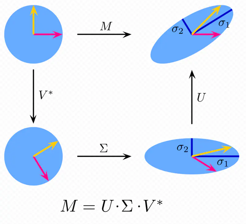
It decomposes any matrix into a rotation, a scaling (based on singular values), and another rotation.
It is a generalization of the eigen value decomposition(for square matrix) to rectangular matrices.
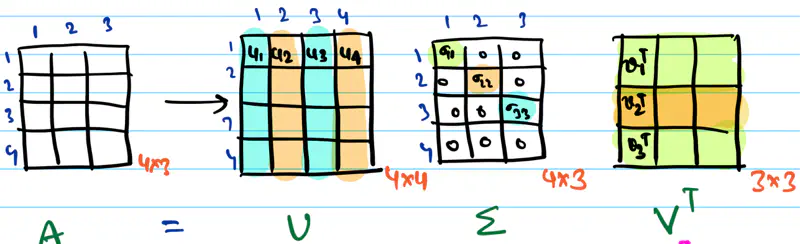
Any rectangular matrix can be decomposed into a product of three matrices using SVD, as follows:
\(\mathbf{U}\): Set of orthonormal eigen vectors of \(\mathbf{AA^T}_{m \times m} \)
\(\mathbf{V}\): Set of orthonormal eigen vectors of \(\mathbf{A^TA}_{n \times n} \)
\(\mathbf{\Sigma}\): Rectangular diagonal matrix, whose diagonal values are called singular values;
square root of non-zero eigen values of \(\mathbf{AA^T}\).
Note: The number of non-zero diagonal entries in \(\mathbf{\Sigma}\) = rank of matrix \(\mathbf{A}\).
Rank (r): Number of linearly independent rows or columns of a matrix.
\( \Sigma = \begin{bmatrix}
\sigma_{11} & 0 & \cdots & 0 \\
\\
0 & \sigma_{22} & \cdots & 0 \\
\vdots & \vdots & \ddots & \vdots \\
\cdots & \cdots & \sigma_{rr} & \vdots \\
0 & 0 & \cdots & 0
\end{bmatrix}
\),
such that, \(\sigma_{11} \geq \sigma_{22} \geq \cdots \geq \sigma_{rr}\), r = rank of \(\mathbf{A}\).
Singular value decomposition, thus refers to the set of scale factors \(\mathbf{\Sigma}\) that are fundamentally
linked to the matrix’s singularity and rank.
- All singular values are non-negative.
- Square roots of the eigen values of the matrix \(\mathbf{AA^T}\) or \(\mathbf{A^TA}\).
- Arranged in non-decreasing order.
\(\sigma_{11} \geq \sigma_{22} \geq \cdots \geq \sigma_{rr} \ge 0\)
Note: If rank of matrix < dimensions, then 1 or more of the singular values are zero, i.e, dimension collapse.
How can we compress the image size to save satellite bandwidth?
We can perform singular value decomposition on the image matrix and find the minimum number of top ranks required to
to successfully reconstruct the original image back.
Say we performed the SVD on the image matrix and found that top 20 rank singular values, out of 1000, are sufficient to
tell what the picture is about.
\(\mathbf{A} = \mathbf{U} \mathbf{\Sigma} \mathbf{V}^T \)
\( = u_1 \sigma_1 v_1^T + u_2 \sigma_2 v_2^T + \cdots + u_r \sigma_r v_r^T \), where \(r = 20\)
A = sum of ‘r=20’ matrices of rank=1.
Now, we need to send only the \(u_i, \sigma_i , v_i\) values for i=20, i.e, top 20 ranks to earth
and then do the calculation to reconstruct the approximation of original image.
\(\mathbf{u} = \begin{bmatrix} u_1 \\ u_2 \\ \vdots \\ u_{1000} \end{bmatrix}\)
\(\mathbf{v} = \begin{bmatrix} v_1 \\ v_2 \\ \vdots \\ v_{1000} \end{bmatrix}\)
So, we need to send data corresponding to 20 (rank=1) matrices, i.e, \(u_i, v_i ~and~ \sigma_i\) = (1000 + 1000 + 1)20 = 200020 pixels (approx)
Therefore, compression rate = (2000*20)/(10^6) = 1/25
- Image compression.
- Low Rank Approximation: Compress data by keeping top rank singular values.
- Noise Reduction: Capture main structure, ignore small singular values.
- Recommendation Systems: Decompose user-item rating matrix to discover underlying user preferences and make recommendations.
The process of approximating any matrix by a matrix of a lower rank, using singular value decomposition.
It is used for data compression.
Any matrix A of rank ‘r’ can be written as sum of rank=1 outer products:
\[ \mathbf{A} = \mathbf{U} \mathbf{\Sigma} \mathbf{V}^T = \sum_{i=1}^{r} \sigma_i \mathbf{u}_i \mathbf{v}_i^T \]\( \mathbf{u}_i : i^{th}\) column vector of \(\mathbf{U}\)
\( \mathbf{v}_i^T : i^{th}\) column vector of \(\mathbf{V}^T\)
\( \sigma_i : i^{th}\) singular value, i.e, diagonal entry of \(\mathbf{\Sigma}\)
Since, the singular values are arranged from largest to smallest, i.e, \(\sigma_1 \geq \sigma_2 \geq \cdots \geq \sigma_r\),
The top ranks capture the vast majority of the information or variance in the matrix.
So, in order to get the best rank-k approximation of the matrix,
we simply truncate the summation after the k’th term.
The approximation \(\mathbf{A_k}\) is called the low rank approximation of \(\mathbf{A}\),
which is achieved by keeping only the largest singular values and corresponding vectors.
Applications:
- Image compression
- Data compression, such as, LoRA (Low Rank Adaptation)
End of Section
6 - Vector & Matrix Calculus
Let \(\mathbf{x} = \begin{bmatrix} x_1 \\ x_2 \\ \vdots \\ x_n \end{bmatrix}_{\text{n×1}}\) be a vector, i.e, \(\mathbf{x} \in \mathbb{R}^n\).
Let \(f(x)\) be a function that maps a vector to a scalar, i.e, \(f : \mathbb{R}^n \rightarrow \mathbb{R}\).
The derivative of function \(f(x)\) with respect to \(\mathbf{x}\) is defined as:
Assumption: All the first order partial derivatives exist.
e.g.:
- \(f(x) = a^Tx\), where,
\(\mathbf{x} = \begin{bmatrix} x_1 \\ x_2 \\ \vdots \\ x_n \end{bmatrix}\),
\(\quad a = \begin{bmatrix} a_1 \\ a_2 \\ \vdots \\ a_n \end{bmatrix}\),
\(\quad a^T = \begin{bmatrix} a_1 & a_2 & \cdots & a_n \end{bmatrix}\)
\(=> f(x) = a^Tx = a_1x_1 + a_2x_2 + \cdots + a_nx_n\)
\(=> \frac{\partial f(x)}{\partial x} = \begin{bmatrix} \frac{\partial x_1}{\partial x} \\ \frac{\partial x_2}{\partial x} \\ \vdots \\ \frac{\partial x_n}{\partial x} \end{bmatrix} \) \(=\begin{bmatrix} a_1 \\ a_2 \\ \vdots \\ a_n \end{bmatrix} = a \)
\( => f'(x) = a \)
- Now, let’s find the derivative for a bit complex, but very widely used function.
\(f(x) = \mathbf{x^TAx} \quad\), where, \(\mathbf{x} = \begin{bmatrix} x_1 \\ x_2 \\ \vdots \\ x_n \end{bmatrix}\), so, \(\quad x^T = \begin{bmatrix} x_1 & x_2 & \cdots & x_n \end{bmatrix}\),
A is a square matrix, \( \mathbf{A} = \begin{bmatrix} a_{11} & a_{12} & \cdots & a_{1k} & \cdots a_{1n} \\ a_{21} & a_{22} & \cdots & a_{2k} & \cdots a_{2n} \\ \vdots & \vdots & \ddots & \vdots & \vdots \\ a_{k1} & a_{k2} & \cdots & a_{kk} & \cdots a_{kn} \\ \vdots & \vdots & \ddots & \vdots & \vdots \\ a_{n1} & a_{n2} & \cdots & a_{nk} & \cdots a_{nn} \end{bmatrix} _{\text{n x n}} \)
So, \( \mathbf{A^T} = \begin{bmatrix} a_{11} & a_{21} & \cdots & a_{k1} & \cdots a_{n1} \\ a_{12} & a_{22} & \cdots & a_{k2} & \cdots a_{n2} \\ \vdots & \vdots & \ddots & \vdots & \vdots \\ a_{1k} & a_{2k} & \cdots & a_{kk} & \cdots a_{nk} \\ \vdots & \vdots & \ddots & \vdots & \vdots \\ a_{1n} & a_{2n} & \cdots & a_{kn} & \cdots a_{nn} \end{bmatrix} _{\text{n x n}} \)
Let’s calculate \(\frac{\partial y}{\partial x_k}\), i.e, for the \(k^{th}\) element and sum it over 1 to n.
The \(k^{th}\) element \(x_k\) will appear 2 times in the below summation, i.e, when \(i=k ~and~ j=k\)
Above, we saw the gradient of a scalar valued function, i.e, a function that maps a vector to a scalar, i.e,
\(f : \mathbb{R}^n \rightarrow \mathbb{R}\).
There is another kind of function called vector valued function, i.e, a function that maps a vector to another vector, i.e,
\(f : \mathbb{R}^n \rightarrow \mathbb{R}^m\).
The Jacobian is the matrix of all first-order partial derivatives of a vector-valued function,
while the gradient is a vector representing the partial derivatives of a scalar-valued function.
- Jacobian matrix provides the best linear approximation of a vector valued function near a given point,
similar to how a derivative/gradient is the best linear approximation for a scalar valued function
Note: Gradient is a special case of the Jacobian;
it is the transpose of the Jacobian for a scalar valued function.
Let, \(f(x)\) be a function that maps a vector to another vector, i.e, \(f : \mathbb{R}^n \rightarrow \mathbb{R}^m\)
\(f(x)_{m \times 1} = \mathbf{A_{m \times n}x_{n \times 1}}\), where,
\(\quad
\mathbf{A} =
\begin{bmatrix}
a_{11} & a_{12} & \cdots & a_{1n} \\
a_{21} & a_{22} & \cdots & a_{2n} \\
\vdots & \vdots & \ddots & \vdots \\
a_{m1} & a_{m2} & \cdots & a_{mn}
\end{bmatrix}
_{\text{m x n}}
\),
\(\mathbf{x} = \begin{bmatrix} x_1 \\ x_2 \\ \vdots \\ x_n \end{bmatrix}_{\text{n x 1}}\),
\(f(x) = \begin{bmatrix} f_1(x) \\ f_2(x) \\ \vdots \\ f_m(x) \end{bmatrix}_{\text{m x 1}}\)
The above matrix is called Jacobian matrix of \(f(x)\).
Assumption: All the first order partial derivatives exist.
Hessian Matrix:
It is a square matrix of second-order partial derivatives of a scalar-valued function.
This is used to characterize the curvature of a function at a give point.
Let, \(f(x)\) be a function that maps a vector to a scalar value, i.e, \(f : \mathbb{R}^n \rightarrow \mathbb{R}\)
The Hessian matrix is defined as:
Note: Most functions in Machine Learning where second-order partial derivatives are continuous, the Hessian is symmetrix.
\( H_{i,j} = H_{j,i} = \frac{\partial f^2(x)}{\partial x_i \partial x_j } = \frac{\partial f^2(x)}{\partial x_j \partial x_i } \)
e.g:
\(f(x) = \mathbf{x^TAx}\), where, A is a symmetric matrix, and f(x) is a scalar valued function.
\(Gradient = \frac{\partial }{\partial x}(\mathbf{x^TAx}) = 2\mathbf{Ax}\), since A is symmetric.
\(Hessian = \frac{\partial^2 }{\partial x^2}(\mathbf{x^TAx}) = \frac{\partial }{\partial x}2\mathbf{Ax} = 2\mathbf{A}\)\(f(x,y) = x^2 + y^2\)
\(Gradient = \nabla f = \begin{bmatrix} \frac{\partial f}{\partial x}\\ \\ \frac{\partial f}{\partial x} \end{bmatrix} = \begin{bmatrix} 2x+0 \\ \\ 0+2y \end{bmatrix} = \begin{bmatrix} 2x \\ \\ 2y \end{bmatrix}\)
\(Hessian = \nabla^2 f = \begin{bmatrix} \frac{\partial^2 f}{\partial x^2} & \frac{\partial^2 f}{\partial x \partial y}\\ \\ \frac{\partial^2 f}{\partial y \partial x} & \frac{\partial^2 f}{\partial y^2} \end{bmatrix} = \begin{bmatrix} 2 & 0 \\ \\ 0 & 2 \end{bmatrix}\)
Let, A is a mxn matrix, i.e \(A \in \mathbb{R}^{m \times n}\)
\(\mathbf{A} =
\begin{bmatrix}
a_{11} & a_{12} & \cdots & a_{1n} \\
a_{21} & a_{22} & \cdots & a_{2n} \\
\vdots & \vdots & \ddots & \vdots \\
a_{m1} & a_{m2} & \cdots & a_{mn}
\end{bmatrix}
_{\text{m x n}}
\)
Let f(A) be a function that maps a matrix to a scalar value, i.e, \(f : \mathbb{R}^{m \times n} \rightarrow \mathbb{R}\)
, then derivative of function f(A) w.r.t A is defined as:
e.g.:
- Let, A is a square matrix, i.e \(A \in \mathbb{R}^{n \times n}\)
and f(A) = trace(A) = \(a_{11} + a_{22} + \cdots + a_{nn}\)
We know that:
\((\frac{\partial f}{\partial A})_{(i,j)} = \frac{\partial f}{\partial a_{ij}}\)
Since, the trace only contains diagonal elements,
=> \((\frac{\partial f}{\partial A})_{(i,j)}\) = 0 for all \(i ⍯ j\)
similarly, \((\frac{\partial f}{\partial A})_{(i,i)}\) = 1 for all \(i=j\)
=> \( \frac{\partial Tr(A)}{\partial A} = \begin{cases} 1, & \text{if } i=j \\ \\ 0, & \text{if } i⍯j \end{cases} \)
\(\frac{\partial f}{\partial A} = \frac{\partial Tr(A)}{\partial A} \begin{bmatrix} 1 & 0 & \cdots & 0 \\ 0 & 1& \cdots & 0 \\ \vdots & \vdots & \ddots & \vdots \\ 0 & 0 & \cdots & 1 \end{bmatrix} = \mathbf{I} \)
Therefore, derivative of trace(A) w.r.t A is an identity matrix.
End of Section
7 - Vector Norms
It is a measure of the size of a vector or distance from the origin.
Vector norm is a function that maps a vector to a real number, i.e, \({\| \cdot \|} : \mathbb{R}^n \rightarrow \mathbb{R}\).
Vector Norm should satisfy following 3 properties:
- Non-Negativity:
Norm is always greater than or equal to zero,
\( {\| x \|} \ge 0\), and \( {\| x \|} = 0\), if and only if \(\vec{x} = \vec{0}\). - Homogeneity (or Scaling):
\( {\| \alpha x \|} = |\alpha| {\| x \|} \). - Triangle Inequality:
\( {\| x + y \|} \le {\| x \|} + {\| y \|} \).
P-Norm:
It is a generalised form of most common family of vector norms, also called Minkowski norm.
It is defined as:
We can change the value of \(p\) to get different norms.
L1 Norm:
It is the sum of absolute values of all the elements of a vector; also known as Manhattan distance.
p=1:
L2 Norm:
It is the square root of the sum of squares of all the elements of a vector; also known as Euclidean distance.
p=2:
L-\(\infty\) Norm:
It is the maximum of absolute values of all the elements of a vector; also known as Chebyshev distance.
p=\(\infty\):
- Let, vector \(\mathbf{x} = \begin{bmatrix} 3 \\ \\ -4 \end{bmatrix}\), then
\({\| x \|_1} = |3| + |-4| = 7\)
\({\| x \|_2} = \sqrt{3^2 + (-4)^2} = \sqrt{25} = 5\)
\({\| x \|_\infty} = max(|3|, |-4|) = max(3, 4) = 4\)
It is a function that assigns non-negative size or magnitude to a matrix.
Matrix Norm is a function that maps a matrix to a non-negative real number, i.e, \({\| \cdot \|} : \mathbb{R}^{m \times n} \rightarrow \mathbb{R}\)
It should satisfy following 3 properties:
- Non-Negativity:
Norm is always greater than or equal to zero,
\( {\| x \|} \ge 0\), and \( {\| x \|} = 0\), if and only if \(\vec{x} = \vec{0}\). - Homogeneity (or Scaling):
\( {\| \alpha x \|} = |\alpha| {\| x \|} \). - Triangle Inequality:
\( {\| x + y \|} \le {\| x \|} + {\| y \|} \).
There are 2 types of matrix norms:
- Element wise norms, e.g,, Frobenius norm
- Vector induced norms Frobenius Norm:
Frobenius Norm:
It is equivalent to the Euclidean norm of the matrix if it were flattened into a single vector.
If A is a matrix of size \(m \times n\), then, Frobenius norm is defined as:
\(\sigma_i\) is the \(i\)th singular value of matrix A.
Vector Induced Norm:
It measures the maximum stretching a matrix can apply when multiplied with a vector,
where the vector has a unit length under the chosen vector norm.
Matrix Induced by Vector P-Norm:
P-Norm:
P=1 Norm:
P=\(\infty\) Norm:
P=2 Norm:
Also called Spectral norm, i.e, maximum factor by which the matrix can stretch a unit vector in Euclidean norm.
Let, matrix \(\mathbf{A} = \begin{bmatrix} a_{11} & a_{12} \\ \\ a_{21} & a_{22} \end{bmatrix}\), then find Frobenius norm.
\({\| A \|_F} = \sqrt{a_{11}^2 + a_{12}^2 + a_{21}^2 + a_{22}^2}\)
\(\mathbf{A}^T = \begin{bmatrix} a_{11} & a_{22} \\ \\ a_{12} & a_{22} \end{bmatrix}\)
=> \(\mathbf{A^TA} = \begin{bmatrix} a_{11} & a_{22} \\ \\ a_{12} & a_{22} \end{bmatrix} \begin{bmatrix} a_{11} & a_{12} \\ \\ a_{21} & a_{22} \end{bmatrix} = \begin{bmatrix} a_{11}^2 + a_{12}^2 & a_{11}.a_{21} + a_{12}.a_{22} \\ \\ a_{21}.a_{11} + a_{22}.a_{12} & a_{21}^2 + a_{22}^2 \end{bmatrix} \)
Therefore, \(Trace(\mathbf{A^TA}) = a_{11}^2 + a_{12}^2 + a_{21}^2 + a_{22}^2\)
=> \({\| A \|_F} = \sqrt{Trace(A^TA)} = \sqrt{a_{11}^2 + a_{12}^2 + a_{21}^2 + a_{22}^2}\)Let, matrix \(\mathbf{A} = \begin{bmatrix} 1 & -2 & 3 \\ \\ 4 & 5 & -6 \end{bmatrix}\), then
Column 1 absolute value sum = |1|+|4| = 5
Column 2 absolute value sum = |-2|+|5|= 7
Column 3 absolute value sum = |3|+|-6|= 9
Row 1 absolute value sum = |1|+|-2|+|3| = 6
Row 2 absolute value sum = |4|+|5|+|-6| = 15
\({\| A \|_1} = max(5,7,9) = 9\) = max column absolute value sum.
\({\| A \|_\infty} = max(6,15) = 15\) = max row absolute value sum.
- Let, matrix \(\mathbf{A} = \begin{bmatrix} 2 & 1 \\ \\ 1 & 2 \end{bmatrix}\), then find spectral norm.
Spectral norm can be found using the singular value decomposition, in order to get the largest singular value.
\({\| A \|_2} = \sigma_{max}(A) \)
\(\mathbf{A} = \mathbf{U \Sigma V^T} \) , where
\(\mathbf{U} = \mathbf{AA^T} \),
\(\mathbf{V} = \mathbf{A^TA} \)
Let’s find the largest eigen value of \(\mathbf{A^TA} \), square root of which will give the largest singular value of \(\mathbf{A}\).
\( \mathbf{V} = \mathbf{A^TA} =
\begin{bmatrix} 2 & 1 \\ \\ 1 & 2 \end{bmatrix}
\begin{bmatrix} 2 & 1 \\ \\ 1 & 2 \end{bmatrix}
= \begin{bmatrix} 5 & 4 \\ \\ 4 & 5 \end{bmatrix}
\)
Now, lets find the eigen values of the above matrix V:
\(det(V-\lambda I) = 0 \)
=> \(
det\begin{bmatrix} 5 - \lambda & 4 \\ \\ 4 & 5- \lambda \end{bmatrix} = 0
\)
=> \( (5 - \lambda)^2 - 16 = 0 \)
=> \( (5 - \lambda) = \pm 4 \)
=> \( (5 - \lambda) = 4 \) or \( (5 - \lambda) = -4 \)
=> \( \lambda = 1 \) or \( \lambda = 9 \)
=> Largest Singular Value = Square root of largest eigen value = \(\sqrt{9} = 3\)
Therefore, \({\| A \|_2} = \sigma_{max}(A) = 3\)
End of Section
8 - Hyperplane
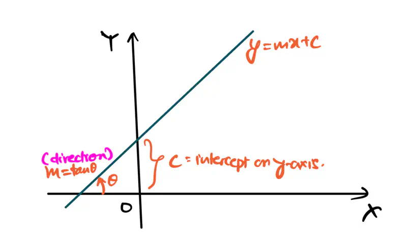
Equation of a line is of the form \(y = mx + c\).
To represent a line in 2D space, we need 2 things:
- m = slope or direction of the line
- c = y-intercept or distance from the origin
Similarly, to represent a hyperplane in d-dimensions, we need 2 things:
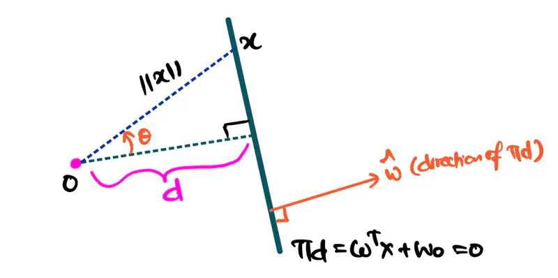
- \(\vec{w}\) = direction of the hyperplane = vector perpendicular to the hyperplane
- \(w_0\) = distance from the origin
Note: There can be only 2 directions of the hyperplane, i.e, direction of a unit vector perpendicular to the hyperplane:
- Towards the origin
- Away from the origin
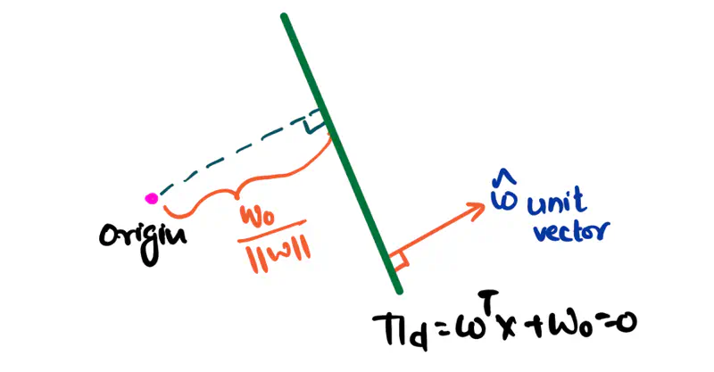
If a point ‘x’ is on the hyperplane, then it satisfies the below equation:
Key Points:
- By convention, the direction of the hyperplane is given by a unit vector perpendicular to the hyperplane , i.e, \({\Vert \mathbf{w} \Vert} = 1\), since the direction is only important.
- \(w_0\) gives the signed perpendicular distance from the origin.
\(w_0 = 0\) => Hyperplane passes through the origin.
\(w_0 < 0\) => Hyperplane is in the same direction of unit vector \(\mathbf{\widehat{w}}\) w.r.t the origin.
\(w_0 > 0\) => Hyperplane is in the opposite direction of unit vector \(\mathbf{\widehat{w}}\) w.r.t the origin.
What is the direction of the hyperplane w.r.t the origin and the direction of the unit vector ?
Equation of a hyperplane is: \(\pi_d = \mathbf{w}^\top \mathbf{x} + w_0 = 0\)
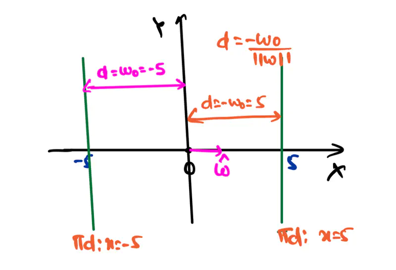
Let, the equation of the line/hyperplane in 2D be:
\(\pi_d = 1.x + 0.y + w_0 = x + w_0 = 0\)
Case 1: \(w_0 < 0\), say \(w_0 = -5\)
Therefore, equation of hyperplane: \( x - 5 = 0 => x = 5\)
Here, the hyperplane(line) is located in the same direction as the unit vector w.r.t the origin,
i.e, towards the +ve x-axis direction.
Case 2: \(w_0 > 0\), say \(w_0 = 5\)
Therefore, equation of hyperplane: \( x + 5 = 0 => x = -5\)
Here, the hyperplane(line) is located in the opposite direction as the unit vector w.r.t the origin,
i.e, towards the -ve x-axis direction.
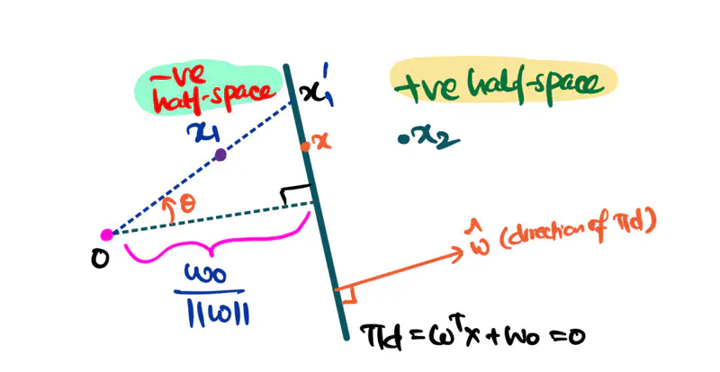
A hyperplane divides a space into 2 distinct parts called half-spaces.
e.g.: A 2D hyperplane divided a 3D space into 2 distinct parts.
Similar example in real world: A wall divides a room into 2 distinct spaces.
Positive Half-Space:
A half space that is in the same direction as the unit vector w.r.t the origin.
Negative Half-Space:
A half space that is in the opposite direction as the unit vector w.r.t the origin.
from equations (1) & (2), we can say that:
\[ \Vert \mathbf{w} \Vert \Vert \mathbf{x_1} \Vert cos{\theta} + w_0 < \Vert \mathbf{w} \Vert \Vert \mathbf{x_1\prime} \Vert cos{\theta} + w_0 \]Everything is same on both the sides except \(\Vert \mathbf{x_1}\Vert\) and \(\Vert \mathbf{x_1\prime\Vert}\), so:
\[ \mathbf{w}^\top \mathbf{x_1} + w_0 < 0 \]i.e, negative half-space, opposite to the direction of unit vector or towards the origin.
Similarly,
i.e, positive half-space, same as the direction of unit vector or away from the origin.
Equation of distance of any point \(x\prime\) from the hyperplane:
The above concept of equation of hyperplane will be very helpful when we discuss the following topics later:
- Logistic Regression
- Support Vector Machines
End of Section