This is the multi-page printable view of this section. Click here to print.
Probability
- 1: Introduction to Probability
- 2: Conditional Probability
- 3: Independence of Events
- 4: Cumulative Distribution Function
- 5: Probability Mass Function
- 6: Probability Density Function
- 7: Expectation
- 8: Moment Generating Function
- 9: Joint & Marginal
- 10: Independent & Identically Distributed
- 11: Convergence
- 12: Law of Large Numbers
- 13: Markov's Inequality
- 14: Cross Entropy & KL Divergence
- 15: Parametric Model Estimation
1 - Introduction to Probability
Because the world around us is very uncertain, and Probability acts as -
the fundamental language
to understand, express and deal with this uncertainty.
- Toss a fair coin, \(P(H) = P(T) = 1/2\)
- Roll a die, \(P(1) = P(2) = P(3) = P(4) = P(5) = P(6) = 1/6\)
- Email classifier, \(P(spam) = 0.95 ,~ P(not ~ spam) = 0.05\)
Range: \([0,1]\)
\(P=0\): Highly unlikely
\(P=1\): Almost certain
Symbol: \(\Omega\)
\(P(\Omega) = 1\)
- Toss a fair coin, sample space: \(\Omega = \{H,T\}\)
- Roll a die, sample space: \(\Omega = \{1,2,3,4,5,6\}\)
- Choose a real number \(x\) from the interval \([2,3]\), sample space: \(\Omega = [2,3]\); sample size = \(\infin\)
Note: There can be infinitely many points between 2 and 3, e.g: 2.21, 2.211, 2.2111, 2.21111, … - Randomly put a point in a rectangular region; sample size = \(\infin\)
Note: There can be infinitely many points in any rectangular region.
A,B,…⊆Ω
- Toss a fair coin, set of possible outcomes: \(\{H,T\}\)
- Roll a die, set of possible outcomes: \(\{1,2,3,4,5,6\}\)
- Roll a die, event \(A = \{1,2\} => P(A) = 2/6 = 1/3\)
- Email classifier, set of possible outcomes: \(\{spam,not ~spam\}\).
- Toss a fair coin, possible outcomes: \(\Omega = \{H,T\}\)
- Roll a die, possible outcomes: \(\Omega = \{1,2,3,4,5,6\}\)
- Choose a real number \(x\) from the interval \([2,3]\) with decimal precision, sample space: \(\Omega = [2,3]\).
Note: There are 99 real numbers between 2 and 3 with 2 decimal precision i.e from 2.01 to 2.99. - Number of cars passing a specific traffic signal in 1 hour.
- A line segment between 2 and 3 - forms a continuum.
- Randomly put a point in a rectangular region.
graph TD
    A[Sample Space] --> |Discrete| B(Finite)
    A --> C(Infinite)
    C --> |Discrete| D(Countable)
C --> |Continuous| E(Uncountable)No overlapping or common outcomes.
If one event occurs, then the other event does NOT occur.
- Roll a die, sample space: \(\Omega = \{1,2,3,4,5,6\}\)
Odd outcome = \(A = \{1,3,5\}\)
Even outcome = \(B = \{2,4,6\}\) are mutually exclusive.
\(P(A \cap B) = 0\)
Since, \(P(A \cup B) = P(A) + P(B) - (P(A \cap B)\)
Therefore, \(P(A \cup B) = P(A) + P(B)\)
Note: If we know that event \(A\) has occurred, then we can say for sure that the event \(B\) did NOT occur.
- Roll a die twice , sample space: \(\Omega = \{1,2,3,4,5,6\}\)
Odd number in 1st throw = \(A = \{1,3,5\}\)
Odd number in 2nd throw = \(B = \{1,3,5\}\)
Note: A and B are independent because whether we get an odd number in 1st roll has NO impact of getting an odd number in second roll.
\(P(A \cap B) = P(A)*P(B)\)
Note: If we know that event \(A\) has occurred, then that gives us NO new information about the event \(B\).
Let’s understand this answer with an example.
Probability of choosing exactly one point on the number line or a real number, say 2.5,
from the interval \([2,3]\) is almost = 0, because there are infinitely many points between 2 and 3.
Also, we can NOT say that choosing exactly 2.5 is impossible, because it exists there on the number line.
But, for all practical purposes, \(P(2.5) = 0\).
Therefore, we say that \(P=0\) means “Highly Unlikely” and NOT “Impossible”.
Extending this line of reasoning, we can say that probability of NOT choosing 2.5, \(P(!2.5) = 1\).
Theoretically yes, because there are infinitely many points between 2 and 3.
But, we cannot say for sure that we cannot choose 2.5 exactly.
There is some probability of choosing 2.5, but it is very small.
Therefore, we say that \(P=1\) means “Almost Sure” and NOT “Certain”.
Here, in this case we can say that \(P(7)=0\) and that means Impossible.
Similarly, we can say that \(P(get ~any ~number ~between ~1 ~and ~6)=1\) and \(P=1 => \) Certain.
End of Introduction
2 - Conditional Probability
It is the probability of an event occurring, given that another event has already occurred.
Allows us to update probability when additional information is revealed.
\(P(A \cap B) = P(A)*P(B \mid A)\)
- Roll a die, sample space: \(\Omega = \{1,2,3,4,5,6\}\)
Event A = Get a 5 = \(\{5\} => P(A) = 1/6\)
Event B = Get an odd number = \(\{1, 3, 5\} => P(B) = 3/6 = 1/2\)
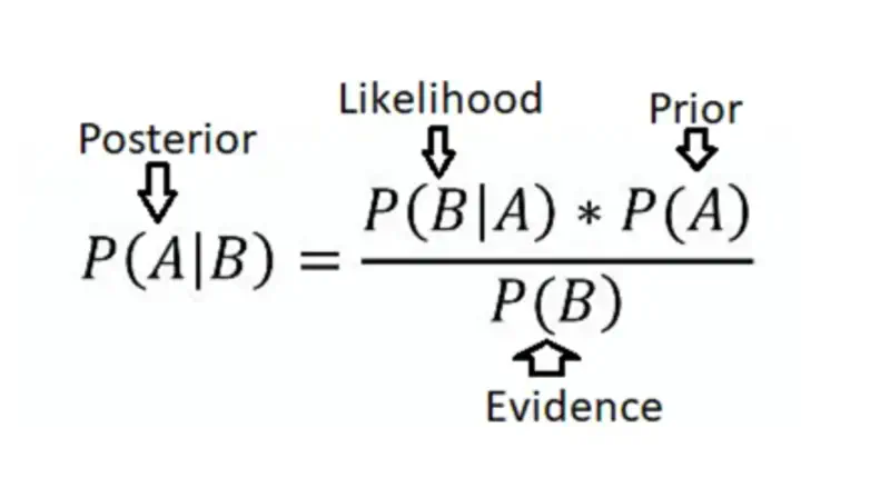
It is a formula that uses conditional probability.
It allows us to update our belief about an event’s probability based on new evidence.
We know from conditional probability and chain rule that:
Combining all the above equations gives us the Bayes’ Theorem:
$$ \begin{aligned} P(A \mid B) = \frac{P(A)*P(B \mid A)}{P(B)} \end{aligned} $$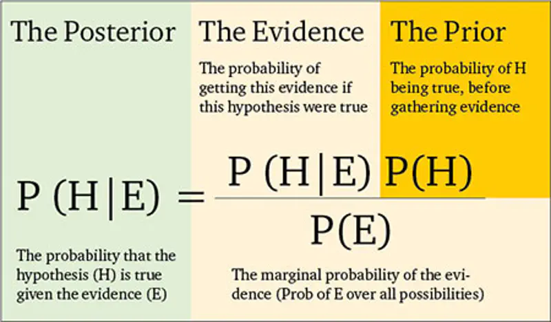
- Roll a die, sample space: \(\Omega = \{1,2,3,4,5,6\}\)
Event A = Get a 5 = \(\{5\} => P(A) = 1/6\)
Event B = Get an odd number = \(\{1, 3, 5\} => P(B) = 3/6 = 1/2\)
Task: Find the probability of getting a 5 given that you rolled an odd number.
\(P(B \mid A) = 1\) = Probability of getting an odd number given that we have rolled a 5.
Now, let’s understand another concept called Law of Total Probability.
Here, we can say that the sample space \(\Omega\) is divided into 2 parts - \(A\) and \(A ^ \complement \)
So, the probability of an event \(B\) is given by:
\[ B = B \cap A + B \cap A ^ \complement \\ P(B) = P(B \cap A) + P(B \cap A ^ \complement ) \\ By ~Chain ~Rule: P(B) = P(A)*P(B \mid A) + P(A ^ \complement )*P(B \mid A ^ \complement ) \]Overall probability of an event B, considering all the different, mutually exclusive ways it can occur.
If A₁, A₂, …, Aₙ are a set of events that partition the sample space, such that they are -
- Mututally exclusive : \(A_i \cap A_j = \emptyset\) for all \(i, j\)
- Exhaustive: \(A₁ \cup A₂ ... \cup Aₙ = \Omega\) for all \(i \neq j\) \[ P(B) = \sum_{i=1}^{n} P(A_i)*P(B \mid A_i) \] where \(n\) is the number of mutually exclusive partitions of the sample space \(\Omega\) .
Now, we can also generalize the Bayes’ Theorem using the Law of Total Probability.
End of Section
3 - Independence of Events
Two events are independent if the occurrence of one event does not affect the probability of the other event.
There are 3 types of independence of events:
- Mutual Independence
- Pair-Wise Independence
- Conditional Independence
Joint probability of two events is equal to the product of the individual probabilities of the two events.
\(P(A \cap B) = P(A)*P(B)\)
Joint probability: The probability of two or more events occurring simultaneously.
\(P(A \cap B)\) or \(P(A, B)\)
- Toss a coin and roll a die -
\(A\) = Get a heads; \(P(A)=1/2\)
\(B\) = Get an odd number; \(P(B)=1/2\)
=> A and B are mutually independent.
Pair-wise independence != Mutual independence.
- Toss 3 coins;
For 2 tosses, sample space: \(\Omega = \{HH,HT, TH, TT\}\)
\(A\) = First and Second toss outcomes are same i.e \(\{HH, TT\}\); \(P(A)= 2/4 = 1/2\)
\(B\) = Second and Third toss outcomes are same i.e \(\{HH, TT\}\); \(P(B)= 2/4 = 1/2\)
\(C\) = Third and First toss outcomes are same i.e \(\{HH, TT\}\); \(P(C)= 2/4 = 1/2\)
Now, pair-wise independence of the above events A & B is - \(P(A \cap B)\)
\(P(A \cap B)\) => Outcomes of first and second toss are same &
outcomes of second and third toss are same.
=> Outcomes of all the three tosses are same.
Total number of outcomes = 8
Desired outcomes = \(\{HHH, TTT\}\) = 2
=> \(P(A \cap B) = 2/8 = 1/4 = P(A) * P(B) = 1/2 * 1/2 = 1/4\)
Therefore, \(A\) and \(B\) are pair-wise independent.
Similarly, we can also prove that \(A\) and \(C\) and \(B\) and \(C\) are also pair-wise independent.
Now, let’s check for mutual independence of the above events A, B & C.
\(P(A \cap B \cap C) = P(A)*P(B)*P(C)\)
\(P(A \cap B \cap C)\) = Outcomes of all the three tosses are same i.e \(\{HHH, TTT\}\)
Total number of outcomes = 8
Desired outcomes = \(\{HHH, TTT\}\) = 2
So, \(P(A \cap B \cap C)\) = 2/8 = 1/4
But, \(P(A)*P(B)*P(C) = 1/2*1/2*1/2 = 1/8\)
Therefore \(P(A \cap B \cap C)\) ≠ \(P(A)*P(B)*P(C)\)
=> \(A, B, C\) are NOT mutually independent but only pair wise independent.
if they are independent given that C has occurred.
Occurrence of C changes the context, causing the events A & B to become independent of each other.
=> A & B are NOT independent.
Now, let’s check for conditional independence of A & B given C.
Therefore, A & B are conditionally independent given C.
End of Section
4 - Cumulative Distribution Function
Random Variable X is represented as, \(X: \Omega \to \mathbb{R} \)
👉 It maps abstract outcomes of a random experiment to concrete numerical values required for mathematical analysis.
- Toss a coin 2 times, sample space: \(\Omega = \{HH,HT, TH, TT\}\)
The above random experiment of coin tosses can be mapped to a random variable \(X: \Omega \to \mathbb{R} \)
\(X: \Omega = \{HH,HT, TH, TT\} \to \mathbb{R}) \)
Say, if we count the number of heads, then
\[ \begin{aligned} X(0) = \{TT\} = 1 \\ X(1) = \{HT, TH\} = 2 \\ X(2) = \{HH\} = 1 \\ \end{aligned} \] Similar, output will be observed for number of tails.
Depending upon the nature of output, random variables are of 2 types - Discrete and Continuous.
Typically obtained by counting.
Discrete random variable cannot take any value between 2 consecutive values.
Possible outcomes are infinite.
- A person’s height in a given range of say 150cm-200cm.
Height can take any value, not just round values, e.g: 150.1cm, 167.95cm, 180.123cm etc.
Now, that we have understood that how random variable can be used to map outcomes of abstract random experiment to real values for mathematical analysis, we will understand its applications.
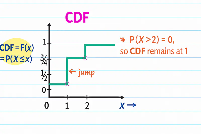
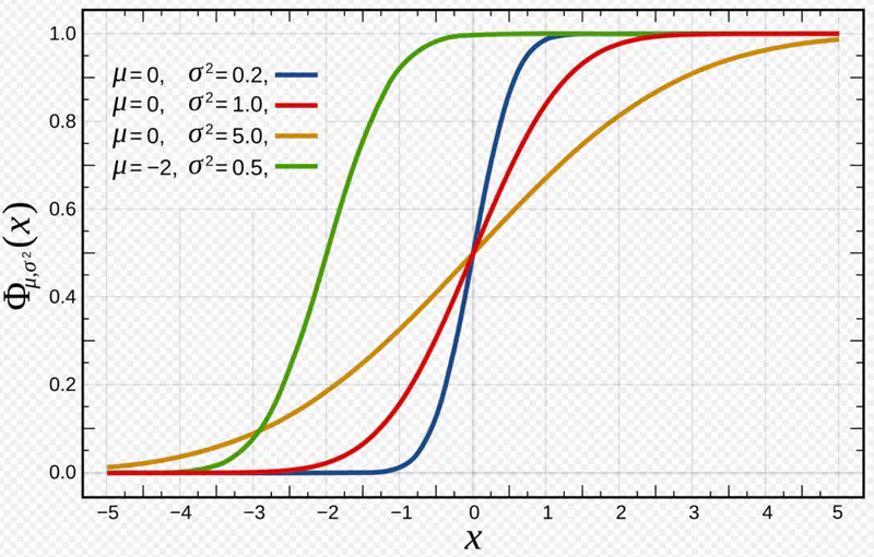
CDF = \(F(X) = P(X \leq x)\) i.e Probability a random variable \(X\) will take for a value \(<=x\).
- Discrete random variable - Toss a coin 2 times, sample space: \(\Omega = \{HH,HT, TH, TT\}\)
Count the number of heads.
\[ \begin{aligned} X(0) = \{TT\} = 1 => P(X = 0) = 1/4 \\ X(1) = \{HT, TH\} = 2 => P(X = 1) = 1/2\\ X(2) = \{HH\} = 1 => P(X = 2) = 1/4 \\ \\ CDF = F(X) = P(X \leq x) \\ F(0) = P(X \leq 0) = P(X < 0) + P(X = 0) = 1/4 \\ F(1) = P(X \leq 1) = P(X < 1) + P(X = 1) = 1/4 + 1/2 = 3/4 \\ F(2) = P(X \leq 2) = P(X < 2) + P(X = 2) = 3/4 + 1/4 = 1 \\ \end{aligned} \]
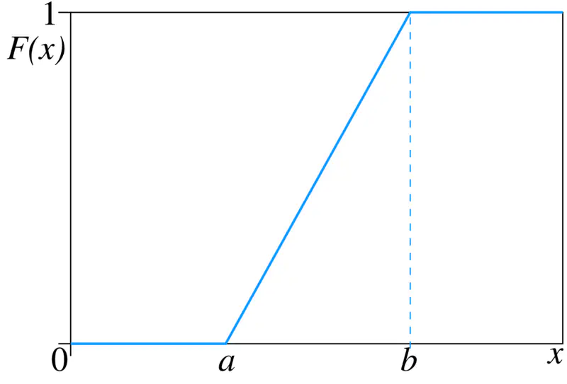
- Continuous random variable - Consider a line segment/interval from \(\Omega = [0,2] \)
Random variable \(X(\omega) = \omega\)
i.e \(X(1) = 1 ~and~ X(1.1) = 1.1 \)
\[ \begin{aligned} P[(0,1/2)] = (1/2)/2 = 1/4 \\ P[(3/4, 2)] = (2-3/4)/2 = 5/8 \\ P(X<=1.1) = P(-\infty, 1.1)/2 = 1.1/2 \end{aligned} \] \[ F_X(x) = P(X \leq x) = \begin{cases} \frac{x}{2} & \text{if } x \in [0,2] \\ 1 & \text{if } x > 2 \\ 0 & \text{if } x < 0 \end{cases} \]
- Non-Decreasing:
For any 2 values \(x_1\) and \(x_2\) such that \(x_1 \leq x_2\), corresponding CDF must satisfy -
\(F(x_1) \leq F(x_2)\)
Note: Cumulative function can never decrease as x increases. - Bounded:
Range of CDF is always between 0 and 1, because CDF represents total probability, which cannot be negative or greater than 1.
\(\lim_{x \to -\infty} F(X) = 0\); as \(x \to -\infty\), event \((X \le x)\) becomes an impossible event
i.e \(P(X \le x) =0\)
\(\lim_{x \to \infty} F(X) = 1\); as \(x \to \infty\), event \((X \le x)\) includes all possible outcomes of the event, making sure that \(P(X \le x) =1\) - Right Continuous:
Function’s value at a point is same as the limit of the function, as we approach that point from right hand side (RHS).
Note: Reason for only right continuity is because how the cumulative distribution function is defined, as we may have a jump on the left side of the point.
\(\lim_{h \to o^+} F(X+h) = F(X)\)
For example:
In the above coin toss CDF example, if we approach X=1 from right, say 1.001, 1.01 etc, the value of \(F(X) = P(X \leq x) = F(1) = 3/4\).
But, if we approach \(X=1\) from left, say 0.99, 0.999 etc, the value of \(F(X) = 1/4\), as these values do NOT yet include the value of the probability at \(X=1\).
Value of the probability of a random variable X, at any given value x, is calculated by summing up all the probabilities for values \(\le x\).
\( CDF = F_X(x) = \sum_{x_i \le x} P(X=x_i) \), where \(P(X=x_i)\) is the Probability Mass Function (PMF) at \(x_i\)
In the above coin toss example -
Height of the jump at ‘x’ = Probability at that value ‘x’.
e.g: Jump at (x=1) = 1/2 = Probability at (x=1).
CDF for continuous random variable is calculated by integrating the probability density function (PDF) from \(-\infty\) to the given value \(x\).
\( CDF = F_X(x) = \int_{-\infty}^{x} f(x) \,dx \), where \(f(x)\) is the Probability Density Function (PDF) of random variable.
Note: We can also say that PDF is the derivative of CDF for continuous random variable.
\(PDF = f(x) = F'(X) = \frac{dF_X(x)}{dx} \)
Read more about Integration
End of Section
5 - Probability Mass Function
It assigns a “non-zero” mass or probability to a specific countable outcome.
Note: Called ‘mass’ because probability is concentrated at a single discrete point.
\(PMF = P(X=x)\)
e.g: Bernoulli, Binomial, Multinomial, Poisson etc.
Commonly visualised as a bar chart.
Note: PMF = Jump at a given point in CDF.
\(PMF = P_x(X=x_i) = F_X(X=x_i) - F_X(X=x_{i-1})\)
- Non-Negative: Probability of any value ‘x’ must be non-negative i.e \(P(X=x) \ge 0 ~\forall x~\).
- Sum = 1: Sum of probabilities of all possible outcomes must be 1.
\( \sum_{x} P(X=x) = 1 \) - For any value that the discrete random variable can NOT take, the probability must be zero.
p = Probability of success
1-p = Probability of failure
Mean = p
Variance = p(1-p)
Note: A single trial that adheres to these conditions is called a Bernoulli trial.
\(PMF, P(x) = p^x(1-p)^{1-x}\), where \(x \in \{0,1\}\)
- Toss a coin, we get heads or tails.
- Result of a test, pass or fail.
- Machine learning, binary classification model.
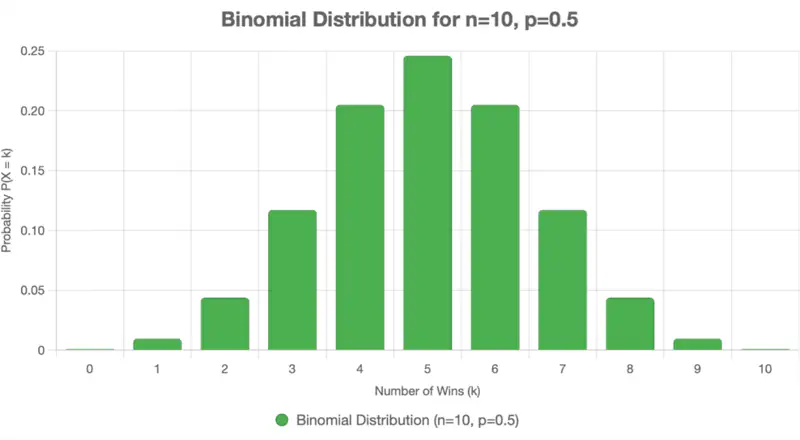
It extends the Bernoulli distribution by modeling the number of successes that occur over a fixed number of
independent trials.
n = Number of trials
k = Number of successes
p = Probability of success
Mean = np
Variance = np(1-p)
\(PMF, P(x=k) = \binom{n}{k}p^k(1-p)^{n-k}\), where \(k \in \{0,1,2,3,...,n\}\)
\(\binom{n}{k} = \frac{n!}{k!(n-k)!}\) i.e number of ways to achieve ‘k’ successes in ‘n’ independent trials.
Note: Bernoulli is a special case of Binomial distribution where n = 1.
Also read about Multinomial distribution i.e where number of possible outcomes is > 2.
- Counting number of heads(success) in ’n’ coin tosses.
- Trials are independent.
- Probability of success remains constant for every trial.
Total number of outcomes in 3 coin tosses = 2^3 = 8
Desired outcomes i.e 2 heads in 3 coin tosses = \(\{HHT, HTH, THH\}\) = 3
Probability of getting exactly 2 heads in 3 coin tosses = \(\frac{3}{8}\) = 0.375
Now lets solve the question using the binomial distribution formula.
Number of successes, k = 1
Number of trials, n = 10
Probability of success, p = 1/3
Probability of winning lottery, P(k=1) =
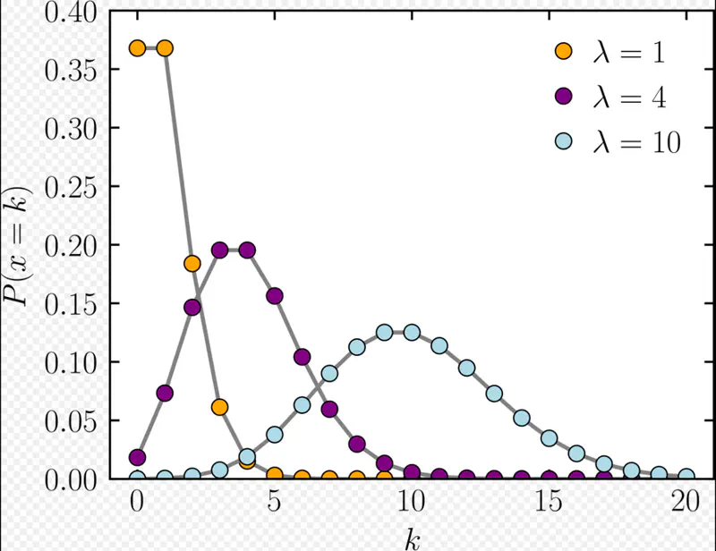
It expresses the probability of an event happening a certain number of times ‘k’ within a fixed interval of time.
Given that:
- Events occur with a known constant average rate.
- Occurrence of an event is independent of the time since the last event.
Parameters:
\(\lambda\): Expected number of events per interval
\(k\) = Number of events in the same interval
Mean = \(\lambda\)
Variance = \(\lambda\)
PMF = Probability of occurrence of ‘k’ events in the same interval
Note: Useful to count data where total population size is large but the probability of an individual event is small.
- Model the number of customers arrival at a service center per hour.
- Number of website clicks in a given time period.
Expected (average) number of emails per hour, \(\lambda\) = 5
Probability of receiving exactly k=3 emails in the next hour =
End of Section
6 - Probability Density Function
This is a function used for continuous random variables to describe the likelihood of the variable taking on a value
within a specific range or interval.
Since, at any given point the probability of a continuous random variable is zero,
we find the probability within a given range.
Note: Called ‘density’ because probability is spread continuously over a range of values
rather than being concentrated at a single point as in PMF.
e.g: Uniform, Gaussian, Exponential, etc.
Note: PDF is a continuous function \(f(x)\).
It is also the derivative of Cumulative Distribution Function (CDF) \(F_X(x)\)
\(PDF = f(x) = F'(X) = \frac{dF_X(x)}{dx} \)
- Non-Negative: Function must be non-negative everywhere i.e \(f(x) \ge 0 \forall x\).
- Sum = 1: Total area under curve must be equal to 1.
\( \int_{-\infty}^{\infty} f(x) \,dx = 1\) - Probability of a continuous random variable in the range [a,b] is given by -
\( P(a \le x \le b) = \int_{a}^{b} f(x) \,dx\)
Consider a line segment/interval from \(\Omega = [0,2] \)
Random variable \(X(\omega) = \omega\)
i.e \(X(1) = 1 ~and~ X(1.1) = 1.1 \)
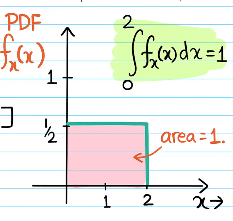
Note: If we know the PDF of a continuous random variable, then we can find the probability of any given region/interval by calculating the area under the curve.
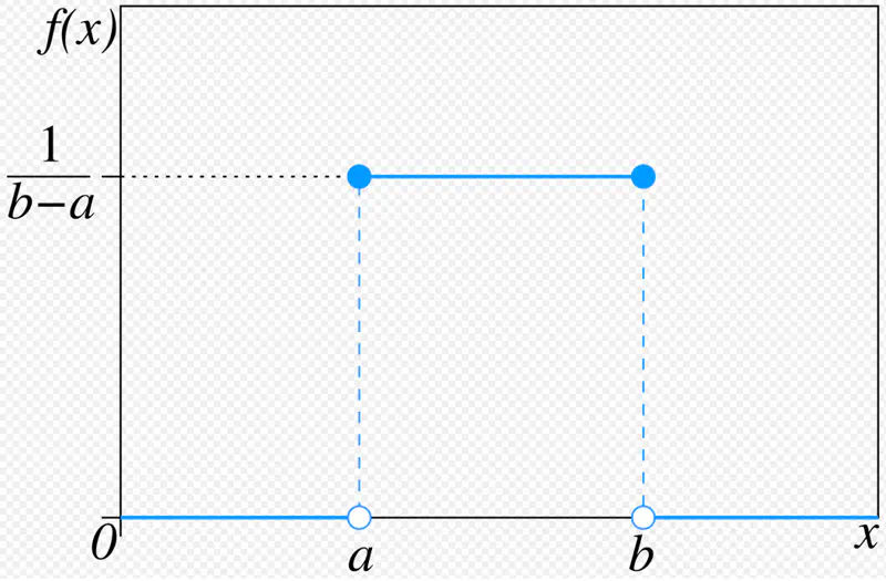
All the outcomes within the given range are equally likely to occur.
Also known as ‘fair’ distribution.
Note: This is a natural starting point to understand randomness in general.
Mean = Median = \( \frac{a+b}{2} ~if~ x \in [a,b] \)
Variance = \( \frac{(b-a)^2}{12} \)
Standard uniform distribution: \( X \sim U(0,1) \)
PDF in terms of mean(\(\mu\)) and standard deviation(\(\sigma\)) -
Random number generator that generates a random number between 0 and 1.
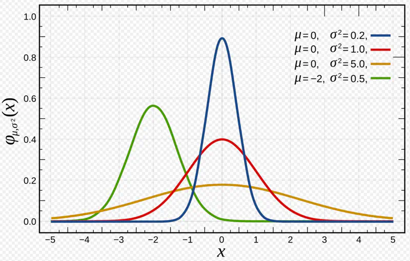
It is a continuous probability distribution characterized by a symmetrical, bell-shaped curve with
most data clustered around the central average, with frequency of values decreasing as they move away from the center.
- Most outcomes are average; extremely low or extremely high values are rare.
- Characterised by mean and standard deviation/variance.
- Peak at mean = median, symmetric around mean.
Note: Most important and widely used distribution.
\[ X \sim N(\mu, \sigma^2) \] $$ \begin{aligned} PDF = f(x) = \dfrac{1}{\sqrt{2\pi}\sigma}e^{-\dfrac{(x-\mu)^2}{2\sigma^2}} \\ \end{aligned} $$
Mean = \(\mu\)
Variance = \(\sigma^2\)
Standard normal distribution:
\[ Z \sim N(0,1) ~i.e~ \mu = 0, \sigma^2 = 1 \]
Any normal distribution can be standardized using Z-score transformation:
- Human height, IQ scores, blood-pressure etc.
- Measurement of errors in scientific experiments.
- 68.27% of the data lie within 1 standard deviation of the mean i.e \(\mu \pm \sigma\)
- 95.45% of the data lie within 2 standard deviations of the mean i.e \(\mu \pm 2\sigma\)
- 99.73% of the data lie within 3 standard deviations of the mean i.e \(\mu \pm 3\sigma\)
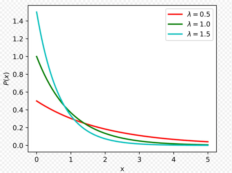
It is used to model the amount of time until a specific event occurs.
Given that:
- Events occur with a known constant average rate.
- Occurrence of an event is independent of the time since the last event.
Parameters:
Rate parameter: \(\lambda\): Average number of events per unit time
Scale parameter: \(\mu ~or~ \beta \): Mean time between events
Mean = \(\frac{1}{\lambda}\)
Variance = \(\frac{1}{\lambda^2}\)
\[ \lambda = \dfrac{1}{\beta} = \dfrac{1}{\mu}\]
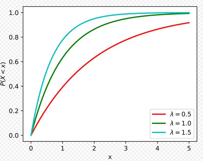
Mean time to serve 1 customer = \(\mu\) = 4 minutes
So, \(\lambda\) = average number of customers served per unit time = \(1/\mu\) = 1/4 = 0.25 minutes
Probability to serve a customer in less than 3 minutes can be found using CDF -
So, probability of a customer being served in less than 3 minutes is 53%(approx).
In this case x = 2 minutes, and \(\lambda\) = 0.25 so,
So, probability of a customer being served in greater than 2 minutes is 60%(approx).
Probability of waiting for an additional period of time for an event to occur is independent of
how long you have already waited.
e.g: Lifetime of electronic items follow exponential distribution.
- Probability of a computer part failing in the next 1 hour is the same regardless of whether
it has been working for 1 day or 1 year or 5 years.
Note: Memoryless property makes exponential distribution particularly useful for -
- Modeling systems that do not experience ‘wear and tear’; where failure is due to a constant random rate rather than degradation over time.
- Also, useful for ‘reliability analysis’ of electronic systems where a ‘random failure’ model is more appropriate than
a ‘wear out’ model.
Task: We want to find the probability of the electronic item lasting for \(x > t+s \) days,
given that it has already lasted for \(x>t\) days.
This is a ‘conditional probability’.
Since,
We want to find: \( P(X > t+s \mid X > t) = ~? \)
Hence, probability that the electronic item will survive for an additional time ’s’ days
is independent of the time ’t’ days it has already survived.
Poisson distribution models the number of events occurring in a fixed interval of time,
given a constant average rate \(\lambda \).
Exponential distribution models the time interval between those successive events.
- 2 faces of the same coin.
- \(\lambda_{poisson}\) is identical to rate parameter \(\lambda_{exponential}\).
Note: If the number of events in a given interval follow a Poisson distribution, then the waiting time between those events will necessarily follow an Exponential distribution.
Lets see the proof for the above statement.
Poisson Case:
The probability of observing exactly ‘k’ events in a time interval of length ’t’
with an average rate of \( \lambda \) events per unit time is given by -
The event that waiting time until next event > t, is same as observing ‘0’ events in that interval.
=> We can use the PMF of Poisson distribution with k=0.
Exponential Case:
Now, lets consider exponential distribution that models the waiting time ‘T’ until next event.
The event that waiting time ‘T’ > t, is same as observing ‘0’ events in that interval.
Observation:
Exponential distribution is a direct consequence of Poisson distribution probability of ‘0’ events.
Using Poisson:
Average failure rate, \(\lambda\) = 1/20 = 0.05
Time interval, t = 10 hours
Number of events, k = 0
Average number of events in interval, (\(\lambda t\)) = (1/20) * 10 = 0.5
Probability of having NO failures in the next 10 hours = ?
Using Exponential:
What is the probability that wait time until next failure > 10 hours?
Waiting time, T > t = 10 hours.
Average number of failures per hour, \(\lambda\) = 1/20 per hour
Therefore, we have seen that this problem can be solved using both Poisson and Exponential distribution.
End of Section
7 - Expectation
Long run average of the outcomes of a random experiment.
When we talk about ‘Expectation’ we mean - on an average.
- Value we expect to get when we repeated an experiment multiple times and took an average of the results.
- Measures the central tendency of a data distribution.
- Similar to ‘Center of Mass’ in Physics.
Note: If the probability of each outcome is different, then we take a weighted average.
Discrete Case:
\(E[X] = \sum_{i=1}^{n} x_i.P(X = x_i) \)
Continuous Case:
\(E[X] = \int_{-\infty}^{\infty} x.f(x) dx \)
if its a tail, then you lose Rs. 50. What is the expected value of the amount that you will win per toss?
Possible outcomes are: \(x_1 = 100 ,~ x_2 = -50 \)
Probability of each outcome is \(P(X = 100) = 0.5,~ P(X = -50) = 0.5 \)
Therefore, the expected value of the amount that you will win per toss is Rs. 25 in the long run.
It is the average of the squared differences from the mean.
- Measures the spread or variability in the data distribution.
- If the variance is low, then the data is clustered around the mean i.e less variability;
and if the variance is high, then the data is widely spread out i.e high variability.
Variance in terms of expected value, where \(E[X] = \mu\), is given by:
\[ \begin{aligned} Var[X] &= E[(X - E[X])^2] \\ &= E[X^2 + E[X]^2 - 2XE[X]] \\ &= E[X^2] + E[X]^2 - 2E[X]E[X] \\ &= E[X^2] + E[X]^2 - 2E[X]^2 \\ Var[X] &= E[X^2] - E[X]^2 \\ \end{aligned} \]Note: This is the computational formula for variance, as it is easier to calculate than the
average of square distances from mean.
PDF of continuous uniform random variable =
$$ \begin{aligned} f_X(x) &= \begin{cases} \dfrac{1}{b-a}, & x \in [a,b] \\ 0, & \text{otherwise.} \end{cases} \\ \end{aligned} $$\[ \begin{aligned} \text{Expected value = mean } = \\[0.5em] E[X] = \dfrac{b+a}{2} \\[0.5em] Var[X] = E[X^2] - E[X]^2 \end{aligned} \]We know \(E[X]\) already, now we will calculate \(E[X^2]\):
\[ \begin{aligned} E[X] &= \int_{-\infty}^{\infty} x.f(x) dx \\ E[X^2] &= \int_{-\infty}^{\infty} x^2.f(x) dx \\ &= \int_{-\infty}^{a} x^2f(x) dx + \int_{a}^{b} x^2f(x) dx + \int_{b}^{\infty} x^2f(x) dx\\ &= 0 + \int_{a}^{b} x^2f(x) dx + 0 \\ &= \int_{a}^{b} x^2f(x) dx \\ &= \dfrac{1}{b-a} \int_{a}^{b} x^2 dx \\ &= \dfrac{1}{b-a} * \{\frac{x^3}{3}\}_{a}^{b} \\ &= \dfrac{1}{b-a} * \{\frac{b^3 - a^3}{3}\} \\ &= \dfrac{1}{b-a} * \{\frac{(b-a)(b^2+ab+a^2)}{3}\} \\ E[X^2] &= \dfrac{b^2+ab+a^2}{3} \end{aligned} \]Now, we know both \(E[X]\) and \(E[X^2]\), so we can calculate \(Var[X]\):
\[ \begin{aligned} Var[X] &= E[X^2] - E[X]^2 \\ &= \dfrac{b^2+ab+a^2}{3} - \dfrac{(b+a)^2}{4} \\ &= \dfrac{b^2+ab+a^2}{3} - \dfrac{b^2+2ab+a^2}{4} \\ &= \dfrac{4b^2+4ab+4a^2-3b^2-6ab-3a^2}{12} \\ &= \dfrac{b^2-2ab+a^2}{12} \\ Var[X]&= \dfrac{(b-a)^2}{12} \end{aligned} \]It is the measure of how 2 variables X & Y vary together.
It gives the direction of the relationship between the variables.
Note: For both direction as well as magnitude, we use Correlation.
Let’s use expectation to compute the co-variance of two random variables X & Y:
Note:
- In a multivariate setting, relationship between all the pairs of random variables are summarized in
a square symmetrix matrix called ‘Co-Variance Matrix’ \(\Sigma\).
- Covariance of a random variable with self gives the variance, hence the diagonals of covariance matrix are variances.
End of Section
8 - Moment Generating Function
They are statistical measures that describe the characteristics of a probability distribution,
such as its central tendency, spread/variability, and asymmetry.
Note: We will discuss ‘raw’ and ‘central’ moments.
Important moments:
- Mean : Central tendency
- Variance : Spread/variability
- Skewness : Asymmetry
- Kurtosis : Tailedness
It is a function that simplifies computation of moments, such as, the mean, variance, skewness, and kurtosis,
by providing a compact way to derive any moment of a random variable through differentiation.
- Provides an alternative to PDFs and CDFs of random variables.
- A powerful property of the MGF is that its \(n^{th}\) derivative, when evaluated at \((t=0)\) = the \(n^{th}\) moment of the random variable.
Not all probability distributions have MGFs; sometimes, integrals may not converge and moment may not exist.
Since, \(MGF = M_X(t) = E[e^{tX}] \), we can write the MGF as:
Say, \( E[X^n] = m_n \), where \(m_n\) is the \(n^{th}\) moment of the random variable, then:
\[ M_X(t) = 1 + \frac{t}{1!}m_1 + \frac{t^2}{2!}m_2 + \frac{t^3}{3!}m_3 + \cdots + \frac{t^n}{n!}m_n + \cdots \\ \]Important: Differentiating \(M_X(t)\) with respect to \(t\), \(i\) times, and setting \((t =0)\) gives us the \(i^{th}\) moment of the random variable.
\[ \frac{dM_X(t) }{dt} = M'_X(t) = 0 + m_1 + \frac{2t}{2!}m_2 + \frac{3t^2}{3!}m_3 + \cdots + \frac{nt^n-1}{n!}m_n + \cdots \\ \]Set \(t=0\), to get the first moment:
\[ \frac{dM_X(t) }{dt} = M'_X(t) = m_1 \]Similarly, second moment = \(M''_X(t) = m_2 = E[X^2]\)
And, \(n^{th}\) derivative = \(M^{(n)}_X(t) = m_n = E[X^n]\)
e.g: \( Var[X] = M''_X(0) - (M'_X(0))^2 \)
Note: If we know the MGF of a random variable, then we do NOT need to do integration or summation to find the moments.
Continuous:
Discrete:
\[ M_X(t) = E[e^{tX}] = \sum_{i=1}^{\infty} e^{tx} P(X=x) \]End of Section
9 - Joint & Marginal
It describes the probability of 2 or more random variables occurring simultaneously.
- The random variables can be from different distributions, such as, discrete and continuous.
Joint CDF:
Discrete Case:
Continuous Case:
Joint PMF:
Key Properties:
- \(P(X = x, Y = y) \ge 0 ~ \forall (x,y) \)
- \( \sum_{i} \sum_{j} P(X = x_i, Y = y_j) = 1 \)
Joint PDF:
Key Properties:
- \(f_{X,Y}(x,y) \ge 0 ~ \forall (x,y) \)
- \( \int_{-\infty}^{\infty} \int_{-\infty}^{\infty} f_{X,Y}(x,y) dy dx = 1 \)
- If we consider 2 random variables, say, height(X) and weight(Y), then the joint distribution will tell us the probability of finding a person having a particular height and weight.
A ball is picked at random from each bag, such that both draws are independent of each other.
Let’s use this example to understand joint probability.
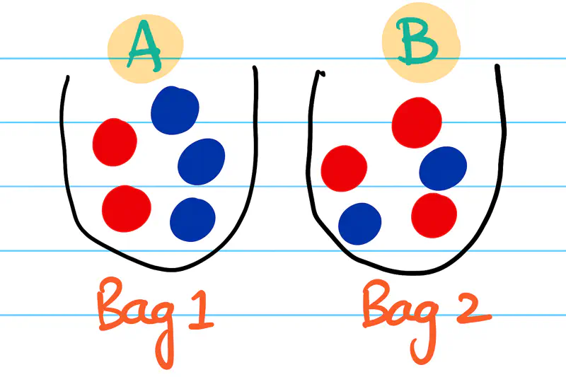
Let A & B be discrete random variables associated with the outcome of the ball drawn from first and second bags
respectively.
| A = Red | A = Blue | |
|---|---|---|
| B = Red | 2/5*3/5 = 6/25 | 3/5*3/5 = 9/25 |
| B = Blue | 2/5*2/5 = 4/25 | 3/5*2/5 = 6/25 |
Since, the draws are independent, joint probability = P(A) * P(B)
Each of the 4 cells in above table shows the probability of combination of results from 2 draws or joint probability.
It describes the probability distribution of an individual random variable in a joint distribution,
without considering the outcomes of other random variables.
- If we have the joint distribution, then we can get the marginal distribution of each random variable from it.
- Marginal probability equals summing the joint probability across other random variables.
Marginal CDF:
We know that Joint CDF =
Marginal CDF =
\[ F_X(a, \infty) = P(X \le a, Y < \infty) = P(X \le a) \]Discrete Case:
Continuous Case:
Law of Total Probability
We know that Joint Probability Distribution =
The events \((Y=y)\) partition the sample space, such that:
- \( (Y=y_1) \cap (Y=y_2) \cap ... \cap (Y=y_n) = \Phi \)
- \( (Y=y_1) \cup (Y=y_2) \cup ... \cup (Y=y_n) = \Omega \)
From Law of Total Probability, we get:
Marginal PMF:
Marginal PDF:
X: Roll a die ; \( \Omega = \{1,2,3,4,5,6\} \)
Y: Toss a coin ; \( \Omega = \{H,T\} \)
Joint PMF = \( P_{X,Y}(x,y) = P(X=x, Y=y) = 1/6*1/2 = 1/12\)
Marginal PMF of X = \( P_X(x) =\sum_{y \in \mathbb{\{H,T\}}} P_{X,Y}(x,y) = = 1/12+1/12 = 1/6\)
=> Marginally, X is uniform over 1-6 i.e a fair die.
Marginal PMF of Y = \( P_Y(y) = \sum_{1}^6 P_{X,Y}(x,y) = 6*(1/12) = 1/2 \)
=> Marginally, Y is uniform over H,T i.e a fair coin.
\( X \sim U(0,1) \)
\( Y \sim U(0,1) \)
Marginal PDF = \(f_X(x) = \int_{-\infty}^{\infty} f_{X,Y}(x,y) dy \)
Joint PDF =
Marginal PDF =
\[ \begin{aligned} f_X(x) &= \int_{0}^{1} f_{X,Y}(x,y) dy \\ &= \int_{0}^{1} 1 dy \\ &= 1 \\ f_X(x) &= \begin{cases} 1 & \text{if } x \in [0,1] \\ 0 & \text{otherwise } \end{cases} \end{aligned} \]There are 2 bags; bag_1 has 2 red balls & 3 blue balls, bag_2 has 3 red balls & 2 blue balls.
A ball is picked at random from each bag, such that both draws are independent of each other.
Let’s use this example to understand marginal probability.
Let A & B be discrete random variables associated with the outcome of the ball drawn from first and second bags
respectively.
| A = Red | A = Blue | P(B) (Marginal) | |
|---|---|---|---|
| B = Red | 2/5*3/5 = 6/25 | 3/5*3/5 = 9/25 | 6/25 + 9/25 = 15/25 = 3/5 |
| B = Blue | 2/5*2/5 = 4/25 | 3/5*2/5 = 6/25 | 4/25 + 6/25 = 10/25 = 2/5 |
| P(A) (Marginal) | 6/25 + 4/25 = 10/25 = 2/5 | 9/25 + 6/25 = 15/25 = 3/5 |
We can see from the table above - P(A=Red) is the sum of joint distribution over all possible values of B i.e Red & Blue.
It measures the probability of an event occurring given that another event has already happened.
- It provides a way to update our belief about the likelihood based on new information.
P(A, B) = Joint Probability of A and B
P(B) = Marginal Probability of B
=> Conditional Probability = Joint Probability / Marginal Probability
Conditional CDF:
Discrete Case:
Continuous Case:
Conditional PMF:
Conditional PDF:
- Generative machine learning models, such as, GANs, learn the conditional distribution of pixels, given the style of input image.
Note: We only have information about the joint and marginal probabilities.
What is the conditional probability of drawing a red ball in the first draw, given that a blue ball is drawn in second draw?
Let A & B be discrete random variables associated with the outcome of the ball drawn from first and second bags
respectively.
A = Red ball in first draw
B = Blue ball in second draw.
| A = Red | A = Blue | P(B) (Marginal) | |
|---|---|---|---|
| B = Red | 6/25 | 9/25 | 3/5 |
| B = Blue | 4/25 | 6/25 | 2/5 |
| P(A) (Marginal) | 2/5 | 3/5 |
Therefore, probability of drawing a red ball in the first draw, given that a blue ball is drawn in second draw = 2/5.
This gives us the conditional expectation of a random variable X, given another random variable Y=y.
Discrete Case:
Continuous Case:
- Conditional expectation of of a person’s weight, given his/her height = 165 cm, will give us the average weight of all people with height = 165 cm.
Applications:
- Linear regression algorithm is conditional expectation of target variable ‘Y’, given input feature variable ‘X’.
- Expectation Maximisation(EM) algorithm is built on conditional expectation.
This gives us the variance of a random variable calculated after taking into account the value(s) of another related variable.
For example:
- Variance of car’s mileage for city driving might be small, but the variance will be large for mix of city and highway driving.
Note: Models that take into account the change in variance or heteroscedasticity tend to be more accurate.
End of Section
10 - Independent & Identically Distributed
Let’s revisit and understand the independence of random variables first.
It means that the knowing the outcome of one random variable does not impact the probability of the other random variable.
Two random variables X & Y are independent if:
- We know that if 2 random variables X,Y are independent, then their covariance is zero,
since there is no linear relationship between them.
- But the converse may NOT be true, i.e, if the covariance is zero, then we can say for sure that the random variables
are independent.
Let’s go through few examples to understand the independence of random variables.
For example:
- Toss a coin + Roll a die.
\[ X = \begin{cases} 1 & \text{if Heads} \\ \\ 0 & \text{if Tails} \end{cases} \\ \text{} \\ Y = \{1,2,3,4,5,6\} \\ \text{} \\ \text{ Joint probability is all possible combinations of X and Y i.e 2x6 = 12 } \\[10pt] \text{ Sample space: } \Omega = \{ (H,1), (H,2), (H,3), (H,4), (H,5), (H,6), \\ (T,1), (T,2), (T,3), (T,4), (T,5), (T,6) \} \]
Here, clearly, X and Y are independent.
- Toss a coin twice.
\(X\) = Number of heads = \(\{0,1,2\}\)
\(Y\) = Number of tails = \(\{0,1,2\}\)
X, Y are NOT independent, but mutually exclusive, because if we know about one, then we automatically know about the other.
- \(X\) is a continuous uniform random variable \( X \sim U(-1,1) \).
\(Y = 2X\).
Let’s check for independence of \(X\) and \(Y\) i.e \(E[XY] = E[X]E[Y]\) or not?
Now, lets calculate the value of \(E[XY]\):
From (1) and (2), we can say that:
\[ E[XY] ⍯ E[X]E[Y] \\ \]Hence, \(X\) and \(Y\) are NOT independent.
Read more about Integration
Similarly, random variables X & Y are said to be identically distributed if they belong to the same probability distribution.
I.I.D assumption for samples(data points) in a dataset means that the samples are:
- Independent, i.e, each sample is independent of the other.
- Identically distributed, i.e, each sample is drawn from the same probability distribution.
- We take the heights of a random sample of people to estimate the average height of the population of a city.
- Here ‘independent’ assumption means that the height of each person in the sample is independent of the other person.
Usually, heights of members of the same family may be highly correlated.
However, for practical purposes, we can assume that all the heights are independent of one another. - And, for ‘identically distributed’ - we can assume that all the heights are from the same Gaussian distribution with some mean and variance.
- Here ‘independent’ assumption means that the height of each person in the sample is independent of the other person.
End of Section
11 - Convergence
A sequence of random variables \(X_1, X_1, \dots, X_n\) is said to converge in probability
to a known random variable \(X\),
if for every number \(\epsilon >0 \), the following is true:
where,
\(X_n\): is the estimator or sample based random variable.
\(X\): is the known or limiting or target random variable.
\(\epsilon\): is the tolerance level or margin of error.
- Toss a fair coin:
Estimator:
\[ X_n = \begin{cases} \frac{n}{n+1} & \text{, if Head } \\ \\ \frac{1}{n} & \text{, if Tail} \\ \end{cases} \]
Known random variable (Bernoulli):
\[ X = \begin{cases} 1 & \text{, if Head } \\ \\ 0 & \text{, if Tail} \\ \end{cases} \]
Say, tolerance level \(\epsilon = 0.1\).
Then,
If n=5;
So, if n=5, then \(|X_n - X| > (\epsilon = 0.1)\).
\( \implies P(|X_n - X| \ge (\epsilon=0.1)) = 1\).
if n=20;
So, if n=20, then \(|X_n - X| < (\epsilon=0.1)\).
\(\implies P(|X_n - X| \ge (\epsilon=0.1)) = 0\).
\( \implies P(|X_n - X| \ge (\epsilon=0.1)) = 0 ~\forall ~n \ge 10\)
Therefore,
Similarly, we can prove that if \(\epsilon = 0.01\), then the probability will be equal to 0 for \( n\ge 100 \).
Note: Task is to check whether the sequence of randome variables \(X_1, X_2, \dots, X_n\) converges in probability to a known random variable \(X\) as \(n\rightarrow\infty\).
So, we can conclude that, if \(n > \frac{1}{\epsilon}\), then:
A sequence of random variables \(X_1, X_2, \dots, X_n\) is said to almost surely converge to a known random variable \(X\),
for \(n \ge 1\), if the following is true:
where,
\(X_n\): is the estimator or sample based random variable.
\(X\): is the known or limiting or target random variable.
If, \(X_n \xrightarrow{Almost ~ Sure} X \), \( \implies X_n \xrightarrow{Probability} X \)
But, converse is NOT true.
*Note: Almost Sure convergence is hardest to satisfy amongst all convergence, such as, convergence in probability,
convergence in distribution, etc.
Read more about Limits
- \(X\) is random variable such that \(X = \frac{1}{2} \), a constant, i.e \(X_1 = X_2 = \dots = X_n = \frac{1}{2}\).
\(Y_1, Y_2,\dots ,Y_n \) are another sequence of random variables, such that :
\[ Y_1 = X_1 \\[10pt] Y_2 = \frac{X_1 + X_2}{2} \\[10pt] Y_3 = \frac{X_1 + X_2 + X_3}{3} \\[10pt] \dots \\ Y_n = \frac{1}{n} \sum_{i=1}^{n} X_i \xrightarrow{Almost ~ Sure} \frac{1}{2} \]
End of Section
12 - Law of Large Numbers
This law states that given a sequence of independent and identically distributed (IID) samples \(X_1, X_1, \dots, X_n\) from a random variable with finite mean, the sample mean (\(\bar{X_n}\)) converges in probability to the expected value \(E[X]\) or population mean (\( \mu \)).
\[ \lim_{n\rightarrow\infty} P(|\bar{X_n} - E[X]| \ge \epsilon) = 0, \forall ~ \epsilon >0 \\[10pt] \\[10pt] \frac{1}{n} \sum_{i=1}^{n} X_i \xrightarrow{Probability} E[X], \text{ as } n \rightarrow \infty \]Note: Does NOT guarantee that sample mean will be close to population mean,
but instead says that - the probability of sample mean being far away from the population mean is low.
Read more about Limits
- Toss a coin large number of times \('n'\), as \(n \rightarrow \infty\), the proportion of heads will probably be very
close to \(0.5\).
However, it does NOT rule out the possibility of a rare sequence, e.g., getting 10 consecutive heads.
But, the probability of such a rare event is extremely low.
This law states that given a sequence of independent and identically distributed (IID) samples \(X_1, X_1, \dots, X_n\) from a random variable with finite mean, the sample mean (\(\bar{X_n}\)) converges almost surely to the expected value \(E[X]\) or population mean (\( \mu \)).
\[ P(\lim_{n\rightarrow\infty} \bar{X_n} = E[X]) = 1, \text{ as } n \rightarrow \infty \\[10pt] \frac{1}{n} \sum_{i=1}^{n} X_i \xrightarrow{Almost ~ Sure} E[X], \text{ as } n \rightarrow \infty \]Note:
- It guarantees that the sequence of sample averages itself converges to population mean, with exception of set of outcomes that has probability = 0.
- Almost certain guarantee; Much stronger statement than Weak Law of Large Numbers.
- Toss a coin large number of times \('n'\), as \(n \rightarrow \infty\), the proportion of heads will converge
to \(0.5\), with probability = 1.
This means that a sequence where the proportion of heads never settles down to 0.5, is a probability = 0 event.
- Almost sure convergence ensures ML model’s reliability by guaranteeing that the average error on a large dataset will
converge to the true error.
Thus, providing confidence that model will perform consistently and accurately on unseen data.
End of Section
13 - Markov's Inequality
It gives an upper bound for the probability that a non-negative random variable will NOT exceed, based on its expected value.
Note: It gives a very loose upper bound.
Read more about Expectation
What is the probability that the restaurant will serve more than 200 customers in the next hour?
Hence, a 25% chance of serving more than 200 customers.
What is the probability that a randomly selected student gets a score of 90 marks or more?
Hence, there is a 78% chance that a randomly selected student gets a score of 90 marks or more.
It states that the probability of a random variable deviating from its mean is small if its variance is small.
- It is a more powerful version of Markov’s Inequality.
- It uses variance of the distribution in addition to the expected value or mean.
- Also, it does NOT assume the random variable to be non-negative.
- It uses more information about the data i.e mean and variance.
Note: It gives a tighter upper bound than Markov’s Inequality.
What is the probability that a randomly selected student gets a score of 90 marks or more?
Given the standard deviation of the test score is 10 marks.
Given, the standard deviation of the test score \(\sigma\) = 10 marks.
=> Variance = \(\sigma^2\) = 100
Hence, Chebyshev’s Inequality gives a far tighter upper bound of 25% than Markov’s Inequality of 78%(approx).
It is an upper bound on the probability that a random variable deviates from its expected value.
It’s an exponentially decreasing bound on the “tail” of a random variable’s distribution,
which can be calculated using its moment generating function.
- It is used for sum or average of independent random variables (not necessarily identically distributed).
- It provides exponentially tighter bounds, better than Chebyshev’s Inequality’s quadratic decay.
- It uses all moments to capture the full shape of the distribution, using the moment generating function(MGF).
Proof:
For the sum of ’n’ independent random variables,
Note: Used to compute how far the sum of independent random variables deviate from their expected value.
Read more about Moment Generating Function
End of Section
14 - Cross Entropy & KL Divergence
It is a measure of the amount of information gained when a specific, individual event occurs, and is defined based on
the probability of that event.
It is defined as the negative logarithm of the probability of the event.
- It is also called ‘Surprisal’.
Note: Logarithm(for base > 1) is a monotonically increasing function, so as x increases, log(x) also increases.
- So, if probability P(x) increases, then surprise factor S(x) decreases.
- Common events have a high probability of occurrence, hence a low surprise factor.
- Rare events have a low probability of occurrence, hence a high surprise factor.
Units:
- The unit of surprise factor with log base 2 is bits.
- with base ’e’ or natural log its nats (natural units of information).
It conveys how much ‘information’ we expect to gain from a random event.
- Entropy is the average or expected value of surprise factor of a random variable.
- More uniform the distribution ⇒ greater average surprise factor, since all possible outcomes are equally likely.
Case 1:
Toss a fair coin; \(P(H) = P(T) = 0.5 = 2^{-1}\)
Surprise factor (Heads or Tails) = \(-log(P(x)) = -log_2(0.5) = -log_2(2^{-1}) = 1~bit\)
Entropy = \( \sum_{x \in X} P(x)log(-P(x)) = 0.5*1 + 0.5*1 = 1 ~bit \)Case 2:
Toss a biased coin; \(P(H) = 0.9 P(T) = 0.1 \)
Surprise factor (Heads) = \(-log(P(x)) = -log_2(0.9) \approx 0.15 ~bits \)
Surprise factor (Tails) = \(-log(P(x)) = -log_2(0.1) \approx 3.32 ~bits\)
Entropy = \( \sum_{x \in X} P(x)log(-P(x)) = 0.9*0.15 + 0.1*3.32 \approx 0.47 ~bits\)
Therefore, a biased coin is less surprising on an average than a fair coin, hence lower entropy.
It is a measure of the average ‘information gain’ or ‘surprise’ when using an imperfect model \(Q\) to encode events
from a true model \(P\).
- It measures how surprised we are on an average, if the true distribution is \(P\), but we predict using another distribution
\(Q\).
A model is trained to classify images as ‘cat’ or ‘dog’. Say, for an input image the true label is ‘cat’,
so the true distribution:
\(P = [1.0 ~(cat), 0.0 ~(dog)]\).
Let’s calculate the cross-entropy for the outputs of 2 models A & B.
Model A:
\(Q_A = [0.8 ~(cat), 0.2 ~(dog)]\)
Cross Entropy = \(H(P, Q_A) = -\sum_{i=1}^n P(x_i)log(Q_A(x_i)) \)
\(= -[1*log_2(0.8) + 0*log_2(0.2)] \approx 0.32 ~bits\)
Note: This is very low cross-entropy, since the predicted value is very close to actual, i.e low surprise.Model B:
\(Q_B = [0.2 ~(cat), 0.8 ~(dog)]\)
Cross Entropy = \(H(P, Q_B) = -\sum_{i=1}^n P(x_i)log(Q_B(x_i)) \)
\(= -[1*log_2(0.2) + 0*log_2(0.8)] \approx 2.32 ~bits\)
Note: Here the cross-entropy is very high, since the predicted value is quite far from the actual truth, i.e high surprise.
It measures the information lost when one probability distribution \(Q\) is used to approximate another distribution \(P\).
It quantifies the ‘extra cost’ in bits needed to encode data using the approximate distribution \(Q\) instead of
the true distribution \(P\).
KL Divergence = Cross Entropy(P,Q) - Entropy(P)
\[ \begin{aligned} D_{KL}(P \parallel Q) &= H(P, Q) - H(P) \\ &= -\sum_{i=1}^n P(x_i)log(Q(x_i)) - [-\sum_{i=1}^n P(x_i)log(P(x_i))] \\[10pt] &= \sum_{i=1}^n P(x_i)[log(P(x_i)) - log(Q(x_i)) ] \\[10pt] D_{KL}(P \parallel Q) &= \sum_{i=1}^n P(x_i)log(\frac{P(x_i)}{Q(x_i)}) \\[10pt] \text{ For continuous case: } \\ D_{KL}(P \parallel Q) &= \int_{-\infty}^{\infty} p(x)log(\frac{p(x)}{q(x)})dx \end{aligned} \]Note:
- If \(P = Q\) ,i.e, P and Q are the same distributions, then KL Divergence = 0.
- KL divergence is NOT symmetrical ,i.e, \(D_{KL}(P \parallel Q) ⍯ (D_{KL}(Q \parallel P)\).
Using the same cat, dog classification problem example as mentioned above.
A model is trained to classify images as ‘cat’ or ‘dog’. Say, for an input image the true label is ‘cat’,
so the true distribution:
\(P = [1.0 ~(cat), 0.0 ~(dog)]\).
Let’s calculate the KL divergence for the outputs of the 2 models A & B.
Let’s calculate entropy first, and we can reuse the cross-entropy values calculated above already.
Entropy: \(H(P) = -\sum_{x \in X} P(x)log(P(x)) = -[1*log_2(1) + 0*log_2(0)] = 0 ~bits\)
Note: \(0*log_2(0) = 0\), is an approximation hack, since \(log(0)\) is undefined.
Model A:
\( D_{KL}(P \parallel Q) = H(P, Q) - H(P) = 0.32 - 0 = 0.32 ~bits \)
Model A incurs an additional 0.32 bits of surprise due to its imperfect prediction.Model B:
\( D_{KL}(P \parallel Q) = H(P, Q) - H(P) = 2.32 - 0 = 2.32 ~bits \)
Model B has much more ‘information loss’ or incurs higher ‘penalty’ of 2.32 bits as its prediction was from from the truth.
It is a smoothed and symmetric version of the Kullback-Leibler (KL) divergence and is calculated by averaging the
KL divergences between each of the two distributions and their combined average distribution.
- Symmetrical and smoothed version of KL divergence.
- Always finite; KL divergence can be infinite if \( P ⍯ 0 ~and~ Q = 0 \).
- Makes JS divergence more stable for ML models where some predicted probabilities may be exactly 0.
Let’s continue the cat and dog image classification example discussed above.
A model is trained to classify images as ‘cat’ or ‘dog’. Say, for an input image the true label is ‘cat’,
so the true distribution:
\(P = [1.0 ~(cat), 0.0 ~(dog)]\).
Step 1: Calculate the average distribution M.
Step 2: Calculate \(D_{KL}(P \parallel M)\).
Step 3: Calculate \(D_{KL}(Q \parallel M)\).
Step 4: Finally, lets put all together to calculate \(D_{JS}(P \parallel Q)\).
Therefore, lower JS divergence value => P and Q are more similar.
End of Section
15 - Parametric Model Estimation
It is the process of finding the best-fitting finite set of parameters \(\Theta\) for a model that assumes a
specific probability distribution for the data.
It involves using the dataset to estimate the parameters (like the mean and standard deviation of a normal distribution)
that define the model.
\(P(X \mid \Theta) \) : Probability of seeing data \(X: (X_1, X_2, \dots, X_n) \), given the parameters \(\Theta\) of the
underlying probability distribution from which the data is assumed to be generated.
Goal of estimation:
We observed data, \( D = \{X_1, X_2, \dots, X_n\} \), and we want to infer the the unknow parameters \(\Theta\)
of the underlying probability distribution, assuming that the data is generated I.I.D.
Read more for I.I.D
Note: Most of the time, from experience, we know the underlying probability distribution of data, such as, Bernoulli, Gaussian, etc.
There are 2 philosophical approaches to estimate the parameters of a parametric model:
- Frequentist:
- Parameters \(\Theta\) is fixed, but unknown, only data is random.
- It views probability as the long-run frequency of events in repeated trials; e.g toss a coin ’n’ times.
- It is favoured when the sample size is large.
- For example, Maximum Likelihood Estimation(MLE), Method of Moments, etc.
- Bayesian:
- Parameters \(\Theta\) itself is unknown, so we model it as a random variable with a probability distribution.
- It views probability as a degree of belief that can be updated with new evidence, i.e. data.
Thus, integrating prior knowledge with data to express the uncertainty about the parameters. - It is favoured when the sample size is small, as it uses prior belief about the data distribution too.
- For example, Maximum A Posteriori Estimation(MAP), Minimum Mean Square Error Estimation(MMSE), etc..
It is the most popular frequentist approach to estimate the parameters of a model.
This method helps us find the parameters \(\Theta\) that make the data most probable.
Likelihood Function:
Say, we have data, \(D = X_1, X_2, \dots, X_n\) are I.I.D discrete random variable with PMF = \(P_{\Theta}(.)\)
Then, the likelihood function is the probability of observing the data, \(D = \{X_1, X_2, \dots, X_n\}\),
given the parameters \(\Theta\).
Task:
Find the value of parameter \(\Theta_{ML}\) that maximizes the likelihood function.
In order to find the parameter \(\Theta_{ML}\) that maximises the likelihood function,
we need to take the first derivative of the likelihood function with respect to \(\Theta\) and equate it to zero.
But, taking derivative of a product is challenging, so we will take the logarithm on both sides.
Note: Log is a monotonically increasing function, i.e, as x increases, log(x) increases too.
Let us denote the log-likelihood function as \(\bar{L}\).
\[ \begin{aligned} \mathcal{\bar{L}_{X_1, X_2, \dots ,X_n}}(\Theta) &= log [\prod_{i=1}^{n} P_{\Theta}(X_i)] \\ &= \sum_{i=1}^{n} log P_{\Theta}(X_i) \\ \end{aligned} \]Therefore, Maximum Likelihood Estimation is the parameter \(\Theta_{ML}\) that maximises the log-likelihood function.
\[ \Theta_{ML}(X_1, X_2, \dots, X_n) = \underset{\Theta}{\mathrm{argmax}}\ \bar{L}_{X_1, X_2, \dots ,X_n}(\Theta) \]Given \(X_1, X_2, \dots, X_n\) are I.I.D. Bernoulli random variable with PMF as below:
Estimate the parameter \(\theta\) using Maximum Likelihood Estimation.
Let, \(n_1 = \) number of 1’s in the dataset.
Likelihood Function:
Log-Likelihood Function:
Maximum Likelihood Estimation:
In order to find the parameter \(\theta_{ML}\), we need to take the first derivative of the log-likelihood function
with respect to \(\theta\) and equate it to zero.
Read more about Derivative
Say, e.g., we have 10 observations for the Bernoulli random variable as: 1,0,1,1,0,1,1,0,1,0.
Then, the parameter \(\Theta_{ML} = \frac{6}{10} = 0.6\) i.e proportion of 1’s.
\(x_1, x_2, \dots, x_n\) are the realisations/observations of the random variable.
Estimate the parameters \(\mu\) and \(\sigma\) of the Gaussian distribution using Maximum Likelihood Estimation.
Likelihood Function:
Log-Likelihood Function:
Note: Here, the first term \( -\frac{n}{2} log (2\pi) \) is a constant wrt both \(\mu\) and \(\sigma\), so we can ignore the term.
Maximum Likelihood Estimation:
Instead of finding \(\mu\) and \(\sigma\) that maximises the log-likelihood function,
we can find \(\mu\) and \(\sigma\) that minimises the negative of the log-likelihood function.
Now, lets differentiate the log likelihood function wrt \(\mu\) and \(\sigma\) separately to get \(\mu_{ML}, \sigma_{ML}\).
Lets, calculate \(\mu_{ML}\) first by taking the derivative of the log-likelihood function wrt \(\mu\) and equating it to 0.
Read more about Derivative
Similarly, we can calculate \(\sigma_{ML}\) by taking the derivative of the log-likelihood function wrt \(\sigma\)
and equating it to 0.
Note: In general MLE is biased, i.e does NOT give an unbiased estimate => divides by \(n\) instead of \((n-1)\).
Bayesian statistics model parameters by updating initial beliefs (prior probabilities) with observed data to form
a final belief (posterior probability) using Bayes’ Theorem.
Instead of a single point estimate, it provides a probability distribution over possible parameter values,
which allows to quantify uncertainty and yields more robust models, especially with limited data.
Bayes’ Theorem:
Read more about Bayes’ Theorem
\(P(\Theta)\): Prior: Initial distribution of \(\Theta\) before seeing the data.
\(P(X \mid \Theta)\): Likelihood: Conditional distribution of data \(X\), given the parameter \(\Theta\).
\(P(\Theta \mid X)\): Posterior: Conditional distribution of parameter \(\Theta\), given the data \(X\).
\(P(X)\): Evidence: Probability of seeing the data \(X\).
\(x_1, x_2, \dots, x_n\) are the realisations, \(\Theta \in [0, 1] \).
Estimate the parameter \(\Theta\) using Bayesian statistics.
Let, \(n_1 = \) number of 1’s in the dataset.
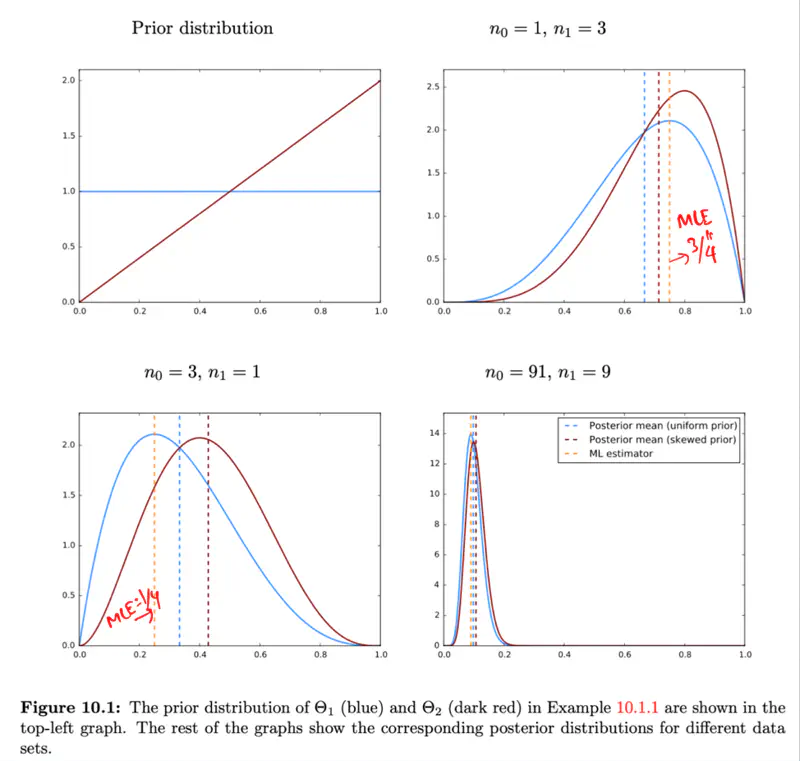
Prior: \(P(\Theta)\) : \(\Theta \sim U(0, 1) \), i.e, parameter \(\Theta\) comes from a continuos uniform
distribution in the range [0,1].
\(f_{\Theta}(\theta) = 1, \theta \in [0, 1] \)
Likelihood: \(P_{X \mid \Theta}(x \mid \theta) = \theta^{n_1} (1 - \theta)^{n - n_1} \).
Posterior:
\[ f_{\Theta \mid X} (\theta \mid x) = \frac{f_{\Theta}(\theta) P_{X \mid \Theta}(x \mid \theta)}{f_{X}(x)} \\ \]Note: The most difficult part is to calculate the denominator \(f_{X}(x)\).
So, either we try NOT to compute it all together, or we try to map it to some known functions to make calculations easier.
We know that we can get the marginal probability by integrating the joint probability over another variable.
Also from conditional probability, we know:
\[ \tag{2} f_{X \mid Y}(x \mid y) = \frac{f_{X,Y}(x,y)}{f_{Y}(y)} \\ => f_{X,Y}(x,y) = f_{Y}(y) f_{X \mid Y}(x \mid y) \]From equations 1 and 2, we have:
\[ \tag{3} f_{X}(x) = \int_{Y}f_{Y}(y) f_{X \mid Y}(x \mid y)dy \]Now let’s replace the value of \(f_{X}(x) \) in the posterior from equation 3:
Posterior:
Beta Function:
It is a special mathematical function denoted by B(a, b) or β(a, b) that is defined by the integral formula:
Note: We can see that the denominator of the posterior is of the form of Beta function.
Posterior:
Suppose, in the above example, we are told that the parameter \(\Theta\) is closer to 1 than 0.
How will we incorporate this useful information (apriori knowledge) into our parameter estimation?
Since, we know apriori that \(\Theta\) is closer to 1 than 0, we should take this initial belief into account
to do our parameter estimation.
Prior:
Posterior:
\[ \begin{aligned} f_{\Theta \mid X} (\theta \mid x) &= \frac{f_{\Theta}(\theta) P_{X \mid \Theta}(x \mid \theta)}{f_{X}(x)} \\[10pt] &= \frac{f_{\Theta}(\theta) P_{X \mid \Theta}(x \mid \theta)}{\int_{\Theta}f_{\Theta}(\theta) P_{X \mid \Theta}(x \mid \theta)d\theta} \\[10pt] &= \frac{f_{\Theta}(\theta) P_{X \mid \Theta}(x \mid \theta)}{\int_{0}^1f_{\Theta}(\theta) P_{X \mid \Theta}(x \mid \theta)d\theta} \\[10pt] \text{ We know that: } f_{\Theta}(\theta) = 2\Theta, \theta \in [0, 1] \\ &= \frac{2\Theta * P_{X \mid \Theta}(x \mid \theta)}{\int_{0}^1 2\Theta* P_{X \mid \Theta}(x \mid \theta)d\theta} \\[10pt] & = \frac{2\Theta * \theta^{n_1} (1 - \theta)^{n - n_1}}{\int_{0}^1 2\Theta * \theta^{n_1} (1 - \theta)^{n - n_1}} \\[10pt] => f_{\Theta \mid X} (\theta \mid x) &= \frac{\theta^{n_1+1} (1 - \theta)^{n - n_1}}{β(n_1+2, n-n_1+1)} \end{aligned} \]Note: If we do NOT have enough data, then we should NOT ignore our initial belief.
However, if we have enough data, then the data will override our initial belief and the posterior will be dominated by data.
Note: Bayesian approach gives us a probability distribution of parameter \(\Theta\).
We can use Bayesian Point Estimators, after getting the posterior distribution, to summarize it with a single value for
practical use, such as,
- Maximum A Posteriori (MAP) Estimator
- Minimum Mean Square Error (MMSE) Estimator
It finds the mode(peak) of the posterior distribution.
- MAP has the minimum probability of error, since it picks single most probable value.
Estimate the unknown parameter \(\mu\) using MAP.
Given that :
\(\Theta\) is discrete, with probability 0.5 for both 0 and 1.
=> The Gaussian distribution is equally likely to be centered at 0 or 1.
Variance: \(\sigma^2 = 1\)
Prior:
Likelihood:
Posterior:
We need to find:
\[ \underset{\Theta}{\mathrm{argmax}}\ P_{\Theta \mid X} (\theta \mid x) \]Taking log on both sides:
Let’s calculate the log-likelihood function first -
\[ \begin{aligned} \log f_{X \mid \Theta}(x \mid \theta) &= \log \prod_{i=1}^n \frac{1}{\sqrt{2\pi}} e^{-\frac{(x_i-\theta)^2}{2}} \\ &= log(\frac{1}{\sqrt{2\pi}})^n + \sum_{i=1}^n \log (e^{-\frac{(x_i-\theta)^2}{2}}), \text{ since \(\sigma = 1\)} \\ &= n\log(\frac{1}{\sqrt{2\pi}}) + \sum_{i=1}^n -\frac{(x_i-\theta)^2}{2} \\ => \tag{2} \log f_{X \mid \Theta}(x \mid \theta) &= n\log(\frac{1}{\sqrt{2\pi}}) - \sum_{i=1}^n \frac{(x_i-\theta)^2}{2} \end{aligned} \]Here computing \(f_{X}(x)\) is difficult.
So, instead of differentiating above equation wrt \(\Theta\), and equating to 0,
we will calculate the above expression for \(\theta=0\) and \(\theta=1\) and compare the values.
This way we can get rid of the common value \(f_{X}(x)\) in both expressions that is not dependent on \(\Theta\).
When \(\theta=1\):
Similarly, when \(\theta=0\):
So, we can say that \(\theta = 1\) only if :
the value of the above expression for \(\theta = 1\) > the value of the above expression for \(\theta = 0\)
From equation 3 and 4:
Note: If the prior is uniform then \(\Theta_{MAP} = \Theta_{MLE}\), because uniform prior does NOT give any information about the initial bias, and all possibilities are equally likely.
What if, in the above example, we know that the initial belief is not uniform but biased towards 0?
Prior:
Now, let’s compare the log-posterior for both the cases i.e \(\theta=0\) and \(\theta=1\) as we did earlier.
But, note that this time the probabilities for \(\theta=0\) and \(\theta=1\) are different.
So, we can say that \(\theta = 1\) only if :
the value of the above expression for \(\theta = 1\) > the value of the above expression for \(\theta = 0\)
From equation 3 and 4 above:
Therefore, we can see that \(\Theta_{MAP}\) is extra biased towards 0.
Note: For a non-uniform prior \(\Theta_{MAP}\) estimate will be pulled towards the prior’s mode.
e.g: Patient has a certain disease or not.
But, what if we want to minimize average magnitude of errors, over time, say predicting a stock’s price?
Just getting to know whether the prediction was right or wrong is not sufficient here.
We also want to know that the prediction was wrong by how much, so that we can minimize the loss over time.
Minimizes the expected value of squared error.
Mean of the posterior distribution is the conditional expectation of parameter \(\Theta\), given the data.
- Posterior mean minimizes the the mean squared error.
\(\hat\Theta(X)\): Predicted value.
\(\Theta\): Actual value.
Let’s revisit the above examples that we used for MLE.
Case 1: Uniform Continuous Prior for parameter \(\Theta\) of Bernoulli distribution
Prior:
Posterior:
Let’s calculate the \(\Theta_{MMSE}\):
Similarly, for the second case where the prior is biased towards 1.
Case 2: Prior is biased towards 1 for parameter \(\Theta\) of Bernoulli distribution
Prior:
Posterior:
So, here in this case our \(\Theta_{MMSE}\) is:
- MMSE is the average of the posterior distribution, whereas MAP is the mode/peak.
- If posterior distribution is symmetric and unimodal (only 1 peak), then MAP and MMSE are very close.
- If posterior distribution is skewed and multimodal (many peaks), then MAP and MMSE can differ a lot.
- MMSE considers all the values of the posterior distribution; hence, it is more accurate than MAP, especially for skewed or multimodal distributions.
End of Section