This is the multi-page printable view of this section. Click here to print.
Statistics
1 - Data Distribution
A single number that describes the central, typical, or representative value of a dataset, e.g, mean, median, and mode.
The mean is the average, the median is the middle value in a sorted list, and the mode is the most frequently occurring value.
- A single representative value can be used to compare different groups or distributions.
The artihmetic average of a set of numbers i.e sum all values and divide by the number of values.
\(mean = \frac{1}{n}\sum_{i=1}^{n}x_i\)
- Most common measure of central tendency.
- Represents the ‘balancing point’ of data.
- Sample mean is denoted by \(\bar{x}\), and population mean by \(\mu\).
Pros:
- Uses all datapoints in its calculation, providing a comprehensive measure.
Cons:
- Highly sensitive to outliers i.e exteme values.
- mean\((1,2,3,4,5) = \frac{1+2+3+4+5}{5} = 3 \)
- With outlier: mean\((1,2,3,4,100) = \frac{1+2+3+4+100}{5} = \frac{110}{5} = 22\)
Note: Just a single extreme value of 100 has pushed the mean from 3 to 22.
The middle value of a sorted list of numbers. It divides the dataset into 2 equal halves.
Calculation:
- Arrange the data points in ascending order.
- If the number of data points is even, the median is the average of the two middle values.
- If the number of data points is odd, the median is the middle value i.e \((\frac{n+1}{2})^{th}\) element.
Pros:
- Not impacted by outliers, making it a more robust/reliable measure, especially for skewed distributions.
Cons:
- Does NOT use all the datapoints in its calculation.
- median\((1,2,3,4,5) = 3\)
- median\((1,2,3,4,5,6) = \frac{3+4}{2} = 3.5\)
- With outlier: median\((1,2,3,4,100) = 3\)
Note: No impact of outlier.
The most frequently occurring value in a dataset.
- Dataset can have 1 mode i.e unimodal, 2 modes i.e bimodal, and more than 2 modes i.e multimodal.
- If NO value repeats, then NO mode.
Pros:
- Only measure of central tendency that can be used for categorical/nominal data, such as, gender, blood group, level of education, etc.
- It can reveal important peaks in data distribution.
Cons:
- A dataset can have multiple modes, or no mode at all, which can make mode less informative.
Quantifies how spread out or scattered the data points are.
E.g: Range, Variance, Standard Deviation, Median Absoulute Deviation(MAD), Skewness, Kurtosis, etc.
The difference between the largest and smallest values in a dataset. Simplest measure of dispersion
\(range = max - min\)
Pros:
- Easy to calculate and understand.
Cons:
- Only considers the the 2 extreme values of dataset and ignores the distribution of data in between.
- Highly sensitive to outliers.
- range\((1,2,3,4,5) = 5 - 1 = 4\)
The average of the squared distance of each value from the mean.
Measures the spread of data points.
\(sample ~ variance = s^2 = \frac{1}{n}\sum_{i=1}^{n}(x_i - \bar{x})^2\)
\(population ~ variance = \sigma^2 = \frac{1}{n}\sum_{i=1}^{n}(x_i - \mu)^2\)
Cons:
- Highly sensitive to outliers, as squaring amplifies the weight of extreme data points.
- Less intuitive to understand, as the units are square of original units.
The square root of the variance, measures average distance of data points from the mean.
- Low standard deviation indicates that the data points are clustered around the mean, whereas
high standard deviation means that the data points are spread out over a wide range.
\(s = sample ~ standard ~ deviation \)
\(\sigma = population ~ standard ~ deviation \)
- Standard Deviation\((1,2,3,4,5) = \sqrt{\frac{1}{n}\sum_{i=1}^{n}(x_i - \bar{x})^2} \) \[ = \sqrt{\frac{1}{5}((1-3)^2 + (2-3)^2 + (3-3)^2 + (4-3)^2 + (5-3)^2)} \\ = \sqrt{\frac{1}{5}(4+1+0+1+4)} \\ = \sqrt{\frac{10}{5}} = \sqrt{2} = 1.414 \]
It is the average of absolute deviation or distance of all data points from mean.
\( mad = \frac{1}{n}\sum_{i=1}^{n}|x_i - \bar{x}| \)
Pros:
- Less sensitive to outliers as compared to standard deviation..
- More intuitive and simpler to understand.
- Mean Absolute Deviation\((1,2,3,4,5) = \\ \frac{1}{5}\left(\left|1-3\right| + \left|2-3\right| + \left|3-3\right| + \left|4-3\right| + \left|5-3\right|\right) = \frac{1}{5}\left(2+1+0+1+2\right) = \frac{6}{5} = 1.2\)
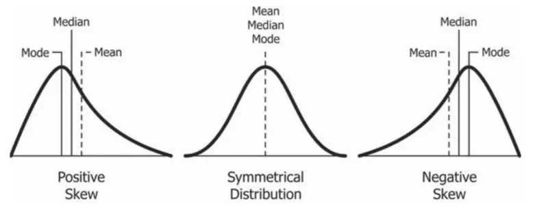
It measures the asymmetry of a data distribution.
Tells us whether the data is concentrated on one side of mean and is there a long tail stretching on the other side.
Positive Skew:
- Tail is longer on the right side of the mean.
- Bulk of data is on the left side of the mean, but there are a few very high values pulling the mean towards the right.
- Mean > Median > Mode.
Negative Skew:
- Tail is longer on the left side of the mean.
- Bulk of data is on the right side of the mean, but there are a few very high values pulling the mean towards the left.
- Mean < Median < Mode.
Zero Skew:
- Perfectly symmetrical like a normal distribution.
- Mean = Median = Mode.
- Consider the salary of employees in a company. Most employees earn a very modest salary, but a few executives earn
extremely high salaries. This dataset will be positively skewed with the mean salary > median salary.
Median salary would be a better representation of the typical salary of employees.
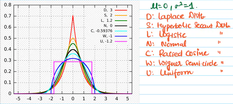
It measures the “tailedness” of a data distribution.
It describes how much the data is concentrated in tails (fat or thin) versus the center.
- It can tell us about the frequency of outliers in the data.
- Thick tails => More outliers.
Excess Kurtosis:
Excess kurtosis is calculated by subtracting 3 from standard kurtosis in order to compare with normal distribution.
Normal distribution has kurtosis = 3.
Mesokurtic:
- Excess kurtosis = 0 i.e normal kurtosis.
- Tails are neither too thick nor too thin.
Leptokurtic:
- High kurtosis, i.e, excess kurtosis > 0 (+ve).
- Heavy or thick tails => High probability of outliers.
- Sharp peak => High concentration of data around mean.
- E.g: Student’s t-distribution, Laplace distribution, etc.
- High risk stock portfolios.
Platykurtic:
- Low kurtosis, i.e, excess kurtosis < 0 (-ve).
- Thin tails => Low probability of outliers.
- Low peak => more uniform distribution of values.
- E.g: Uniform distribution, Bernoulli(P=0.5) distribution, etc.
- Investment in fixed deposits.
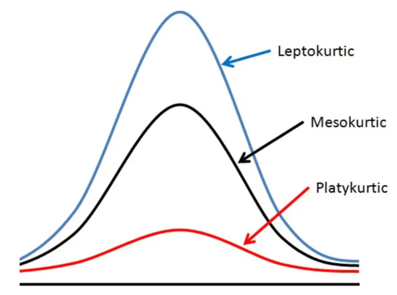
E.g: Percentile, Quartile, Inter Quartile Range(IQR), etc.
It indicates the percentage of scores in a dataset that are equal to or below a specific value.
Here, the complete dataset is divided into 100 equal parts.
- \(k^{th}\) percentile => at least \(k\) percent of the data points are equal to or below the value.
- It is a relative comparison, i.e, compares a score with the entire group’s performance.
- Quartiles are basis for box plots.
- 90th percentile => score is higher than 90% of of all other test takers.
They are special percentiles that divide the complete dataset into 4 equal parts.
Q1 => 25th percentile, value below which 25% of the data falls.
Q2 => 50th percentile, value below which 50% of the data falls; median.
Q3 => 75th percentile, value below which 75% of the data falls.
- Data = \(\{1,2,3,4,5,6,7,8,9,10,100\}\) \[ Q1 = (11+1) * 1/4 = 12*1/4 = 3 \\ Q2 = (11+1) * 1/2 = 12*1/2 = 6 \\ Q3 = (11+1) * 3/4 = 12*3/4 = 9 \]
It is the single number that measures the spread of middle 50% of the data, i.e Q1-Q3.
- More robust measure of spread than range as is NOT impacted by outliers.
IQR = Q3 - Q1
- Data = \(\{1,2,3,4,5,6,7,8,9,10,100\}\) \[ Q1 = (11+1) * 1/4 = 12*1/4 = 3 \\ Q2 = (11+1) * 1/2 = 12*1/2 = 6 \\ Q3 = (11+1) * 3/4 = 12*3/4 = 9 \]
Therefore, IQR = Q3-Q1 = 9-3 = 6
IQR is a standard tool for detecting outliers.
Values that fall outside the ‘fences’ can be considered as potential outliers.
Lower fence = Q1 - 1.5 * IQR
Upper fence = Q3 + 1.5 * IQR
- Data = \(\{1,2,3,4,5,6,7,8,9,10,100\}\) \[ Q1 = (11+1) * 1/4 = 12*1/4 = 3 \\ Q2 = (11+1) * 1/2 = 12*1/2 = 6 \\ Q3 = (11+1) * 3/4 = 12*3/4 = 9 \]
IQR = Q3-Q1 = 9-3 = 6
Lower fence = Q1 - 1.5 * IQR = 3 - 9 = -6
Upper fence = Q3 + 1.5 * IQR = 9 + 9 = 18
So, any data point that is less than -6 or greater than 18 is considered as a potential outlier.
As in this example, 100 can be considered as an outlier.
Even though the above metrics give us a good idea of the data distribution,
but still we should always plot the data and visually inspect the data distribution.
As these metrics may not provide the complete picture.
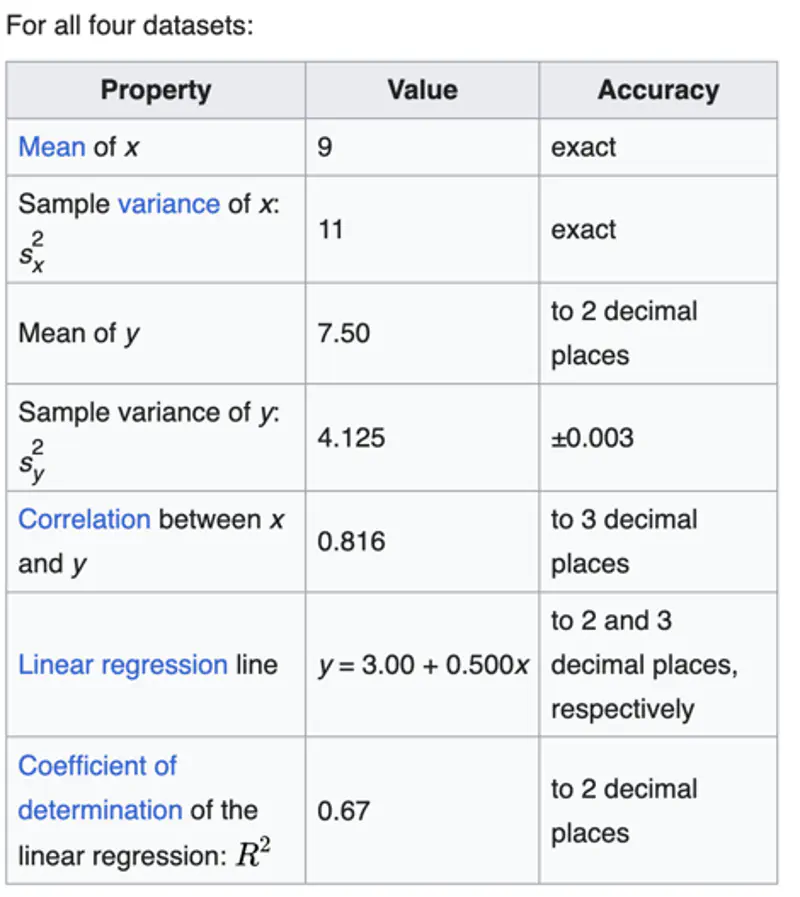
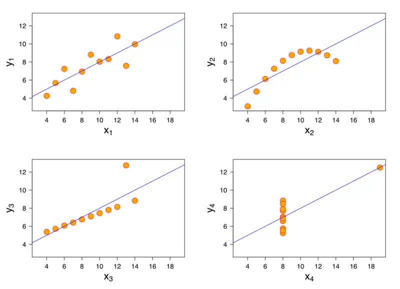
A mathematician called Francis John Anscombe has illustrated this point beautifully in his Anscombe’s Quartet.
Anscombe’s quartet:
It comprises four datasets that have nearly identical simple descriptive statistics,
yet have very different distributions and appear very different when plotted.
End of Section
2 - Correlation
It measures the direction of linear relationship between two variables \(X\) and \(Y\).
\(N\) = size of population
\(\mu_{x}\) = population mean of \(X\)
\(\mu_{y}\) = population mean of \(Y\)
\(n\) = size of sample
\(\bar{x}\) = sample mean of \(X\)
\(\bar{y}\) = sample mean of \(Y\)
Note: We have a term (n-1) instead of n in the denominator to make it an unbiased estimate, called Bessel’s Correction.
If both \((x_i - \bar{x})\) and \((y_i - \bar{y})\) have the same sign, then the product is positive(+ve).
If both \((x_i - \bar{x})\) and \((y_i - \bar{y})\) have opposite signs, then the product is negative(-ve).
The final value of covariance depends on the sum of the above individual products.
\( \begin{aligned} \text{Cov}(X, Y) &> 0 &&\Rightarrow \text{ } X \text{ and } Y \text{ increase or decrease together} \\ \text{Cov}(X, Y) &= 0 &&\Rightarrow \text{ } \text{No linear relationship} \\ \text{Cov}(X, Y) &< 0 &&\Rightarrow \text{ } \text{If } X \text{ increases, } Y \text{ decreases (and vice versa)} \end{aligned} \)
Limitation:
Covariance is scale-dependent, i.e, units of X and Y impact its magnitude.
This makes it hard to make comparisons of covariance across different datasets.
E.g: Covariance between age and height will NOT be same as the covariance between years of experience and salary.
Note:It only measures the direction of the relationship, but does NOT give any information about the strength of the relationship.
- \(X = [1, 2, 3] \) and \(Y = [2, 4, 6] \)
Let’s calculate the covariance:
\(\text{Cov}(X, Y) = \frac{1}{n-1}\sum_{i=1}^{n}(x_i - \bar{x})(y_i - \bar{y})\)
\(\bar{x} = 2\) and \(\bar{y} = 4\)
\(\text{Cov}(X, Y) = \frac{1}{3-1}[(1-2)(2-4) + (2-2)(4-4) + (3-2)(6-4)]= 0\)
\( = \frac{1}{2}[2+0+2]= 2\)
=> Cov(X,Y) > 0 i.e if X increases, Y increases and vice versa.
It measures both the strength and direction of the linear relationship between two variables \(X\) and \(Y\).
It is a standardized version of covariance that gives a dimensionless measure of linear relationship.
There are 2 popular ways to calculate correlation coefficient:
- Pearson Correlation Coefficient (r)
- Spearman Rank Correlation Coefficient (\(\rho\))
It is a standardized version of covariance and most widely used measure of correlation.
Assumption: Data is normally distributed.
\(\sigma_{x}\) and \(\sigma_{y}\) are the standard deviations of \(X\) and \(Y\).
Range of \(r\) is between -1 and 1.
\(r = 1\) => perfect +ve linear relationship between X and Y
\(r = -1\) => perfect -ve linear relationship between X and Y
\(r = 0\) => NO linear relationship between X and Y.
Note: A correlation coefficient of 0.9 means that there is a strong linear relationship between X and Y,
irrespective of their units.
- \(X = [1, 2, 3] \) and \(Y = [2, 4, 6] \)
Let’s calculate the covariance:
\(\text{Cov}(X, Y) = \frac{1}{n-1}\sum_{i=1}^{n}(x_i - \bar{x})(y_i - \bar{y})\)
\(\bar{x} = 2\) and \(\bar{y} = 4\)
\(\text{Cov}(X, Y) = \frac{1}{3-1}[(1-2)(2-4) + (2-2)(4-4) + (3-2)(6-4)]= 0\)
\( => \text{Cov}(X, Y) = \frac{1}{2}[2+0+2]= 2\)
Let’s calculate the standard deviation of \(X\) and \(Y\):
\(\sigma_{x} = \sqrt{\frac{1}{n-1}\sum_{i=1}^{n}(x_i - \bar{x})^2} \)
\(= \sqrt{\frac{1}{3-1}[(1-2)^2 + (2-2)^2 + (3-2)^2]}\)
\(= \sqrt{\frac{1+0+1}{2}} =\sqrt{\frac{2}{2}} = 1 \)
Similarly, we can calculate the standard deviation of \(Y\):
\(\sigma_{y} = \sqrt{\frac{1}{n-1}\sum_{i=1}^{n}(y_i - \bar{y})^2} \)
\(= \sqrt{\frac{1}{3-1}[(2-4)^2 + (4-4)^2 + (6-4)^2]}\)
\(= \sqrt{\frac{4+0+4}{2}} =\sqrt{\frac{8}{2}} = 2 \)
Now, we can calulate the pearson correlation coefficient (r):
\(r_{xy} = \frac{Cov(X, Y)}{\sigma_{x} \sigma_{y}}\)
=> \(r_{xy} = \frac{2}{1* 2}\)
=> \(r_{xy} = 1\)
Therefore, we can say that there is a strong +ve linear relationship between X and Y.
It is a measure of the strength and direction of the monotonic relationship between two ranked variables \(X\) and \(Y\).
It captures monotonic relationship, meaning the variables move in the same or opposite direction,
but not necessarily a linear relationship.
- It is used when Pearson’s correlation is not suitable, such as, ordinal data, or when the continuous data does not meet the assumptions of linear methods, such as, Pearson’s correlation.
- Non-parametric measure of correlation that uses ranks instead of raw data.
- Quantifies how well the ranks of one variable predict the ranks of the other variable.
- Range of \(\rho\) is between -1 and 1.
- Compute the correlation of ranks awarded to a group of 5 students by 2 different teacherrs.
Student Teacher A Rank Teacher B Rank \(d_i\) \(d_i^2\) S1 1 2 -1 1 S2 2 1 1 1 S3 3 3 0 0 S4 4 5 -1 1 S5 5 4 1 1
\(\sum_{i}d_i^2 = 4 \)
\( n = 5 \)
\(\rho_{xy} = 1 - \frac{6\sum_{i}d_i^2}{n(n^2-1)}\)
=> \(\rho_{xy} = 1 - \frac{6*4}{5(5^2-1)}\)
=> \(\rho_{xy} = 1 - \frac{24}{5*24}\)
=> \(\rho_{xy} = 1 - \frac{1}{5}\)
=> \(\rho_{xy} = 0.8\)
Therefore, we can say that there is a strong +ve correlation between the ranks given by teacher A and teacher B.
- \(X = [1, 2, 3] \) and \(Y = [1, 8, 27] \)
Here, Spearman’s rank correlation coefficient \(\rho\) will be perfect 1 as there is a monotonic relationship i.e as X increases, Y increases and vice versa.
But, the Pearson’s correlation coefficient (r) will be slightly less than 1 i.e r = 0.9662.
Correlation is very useful in feature selection for training machine learning models.
- If 2 features are highly correlated => they provide redundant information.
- One of the features can be removed without significant loss of information.
- Keeping both can cause issues, such as, multicollinearity.
- If a feature is highly correlated with the target variable => this feature is a strong predictor, so keep it.
- A feature with very low or near zero correlation with the target variable may be considered for removal, as they have little predictive power.
Causation means that one variable directly causes the change in another variable, i.e, direct
cause->effect relationship.
Whereas, correlation means that two variables move together.
- Correlation does NOT imply Causation.
- Correlation simply shows an association between two variables that could be coincidental or due to some third, unobserved, factor.
E.g: Election results and stock market - there may be some correlation between the two,
but establishing clear causal links is difficult.
End of Section
3 - Central Limit Theorem
It is the true average of the entire group.
It describe the central tendency of the entire population.
\( \mu = \frac{1}{N}\sum_{i=1}^{N}x_i \)
N: Number of data points
It is the average of a smaller representative subset (a sample) of the entire population.
It provides an estimate of the population mean.
\( \bar{x} = \frac{1}{n}\sum_{i=1}^{n}x_i \)
n: size of sample
the sample mean converges to the true the population mean.
In other words, a long-run average of a repeated random variable approaches the expected value.
This law states that for a sequence of of I.I.D random variables \( X_1, X_2, \dots, X_n \),
with finite mean and variance, the distribution of the sample mean \( \bar{X} \) approaches a normal distribution
as \( n \rightarrow \infty \), regardless of its original population distribution.
The distribution of the sample mean is : \( \bar{X} \sim N(\mu, \sigma^2/n)\)
Let, \( X_1, X_2, \dots, X_n \) are I.I.D random variables.
- Population mean = \(E[X_i] = \mu < \infty\)
- Population Variance = \(Var[X_i] = \sigma^2 < \infty \)
- Sample mean = \( \bar{X_n} = \frac{1}{n}\sum_{i=1}^{n}X_i = \frac{1}{n}(X_1 + X_2+ \dots +X_n) \)
- Variance of sample means = \( Var[\bar{X_n}] = Var[\frac{1}{n}(X_1+ X_2+ \dots+ X_n)]\)
Now, let’s calculate the variance of sample means.
We know that:
- \(Var[X+Y] = Var[X] + Var[Y] \), for independent random variables X and Y.
- \(Var[cX] = c^2Var[X] \), for constant ‘c’.
Let’s apply above 2 rules on the variance of sample means equation above:
\[ \begin{aligned} Var[\bar{X_n}] &= Var[\frac{1}{n}(X_1+ X_2+ \dots+ X_n)] \\ &= \frac{1}{n^2}[Var[X_1+ X_2+ \dots+ X_n]] \\ &= \frac{1}{n^2}[Var[X_1] + Var[X_2] + \dots + Var[X_n]] \\ \text{We know that: } Var[X_i] = \sigma^2 \\ &= \frac{1}{n^2}[\sigma^2 + \sigma^2 + \dots + \sigma^2] \\ &= \frac{n\sigma^2}{n^2} \\ => Var[\bar{X_n}] &= \frac{\sigma^2}{n} \end{aligned} \]Since, standard deviation = \(\sigma = \sqrt{Variance}\)
Therefore, Standard Deviation\([\bar{X_n}] = \sqrt{\frac{\sigma^2}{n}} = \frac{\sigma}{\sqrt{n}}\)
The standard deviation of the sample means is also known as “Standard Error”.
Note: We can also standardize the sample mean, i.e, mean centering and variance scaling.
Standardisation helps us to use the Z-tables of normal distribution.
We know that, a standardized random variable \(Y_i = \frac{X_i - \mu}{\sigma}\)
Similarly, standardized sample mean:
Note: For practical purposes, \(n \ge 30\) is considered as a sufficient sample size for the CLT to hold.
- Let’s collect the data for height of people in a city to find the average height of people in the city.
- Sample size (n) = 100
- And then repeat this data collection process 1000 times.
- For each of these 1000 (k) samples, calculate the sample mean \(X_1, X_2, \dots, X_{1000(k)} \)
- Now, when we plot these 1000(k) sample means, the resulting distribution will be very close to a normal/Gaussian distribution.
\(\bar{X_n} \sim N(\mu, \sigma^2/n)\), for large n, typically \(n \ge 30\).
Note:
- ‘k’ = a large number of repetitions allows us to observe the distribution of sample means after plotting.
- ’n’ = number of samples in each repetition is fixed for any given calculation of sample mean \(\bar{X_n}\).
The variance must be finite, else, the sample mean will NOT converge to a normal distribution.
If a distribution has a heavy tail, then the expected value calculation diverges.
e.g:
- Cauchy distribution has infinite mean and infinite variance.
- Pareto distribution (with low alpha) has infinite variance, such as distribution of wealth.
End of Section
4 - Confidence Interval
It is a range of values that is likely to contain the true population mean, based on a sample.
Instead of giving a point estimate, it gives a range of values with confidence level.
For normal distribution, confidence interval :
\(\bar{X}\): Sample mean
\(Z\): Z-score corresponding to confidence level
\(n\): Sample size
\( \sigma \): Population Standard Deviation
Applications:
- A/B testing, i.e., compare 2 or more versions of a product.
- ML model performance evaluation, i.e, instead of giving a single performance score of say 85%,
it is better to provide a 95% confidence interval, such as, [82.5%, 87.8%].
95% confidence interval does NOT mean there is a 95% chance that the true mean lies in the specific calculated interval.
- It just means that if we repeat the sampling process many times, then 95% of of those calculated intervals will capture or contain the true population mean \(\mu\).
- Also, we cannot say there is 95% probability that the true mean is within that specific range because true population mean is a fixed constant, NOT a random variable.
Let’s suppose we want to measure the average weight of a certain species of dog.
We want to estimate the true population
mean \(\mu\) using confidence interval.
Note: True average weight = 30 kg, but this is NOT known to us.
| Sample Number | Sample Mean | 95% Confidence Interval | Did it capture \(\mu\) ? |
|---|---|---|---|
| 1 | 29.8 kg | (28.5, 31.1) | Yes |
| 2 | 30.4 kg | (29.1, 31.7) | Yes |
| 3 | 31.5 kg | (30.2, 32.8) | No |
| 4 | 28.1 kg | (26.7, 29.3) | No |
| - | - | - | - |
| - | - | - | - |
| - | - | - | - |
| 100 | 29.9 kg | (28.6, 31.2) | Yes |
- We generated 100 confidence intervals(CI) each based on different samples.
- 95% CI guarantees that, in long run, 95 out of 100 CIs will include the true average weight, i.e, \(\mu=30kg\), and may be will miss 5 out of 100 times.
Suggest which company is offering a better salary?
Below is the details of the salaries based on a survey of 50 employees.
| Company | Average Salary(INR) | Standard Deviation |
|---|---|---|
| A | 36 lpa | 7 lpa |
| B | 40 lpa | 14 lpa |
For comparison, let’s calculate the 95% confidence interval for the average salaries of both companies A and B.
We know that:
\( CI = \bar{X} \pm Z\frac{\sigma}{\sqrt{n}} \)
Margin of Error(MoE) \( = Z\frac{\sigma}{\sqrt{n}} \)
Z-Score for 95% CI = 1.96
\(MoE_A = 1.96*\frac{7}{\sqrt{50}} \approx 1.94 \)
=> 95% CI for A = \(36 \pm 1.94 \) = [34.06, 37.94]
\(MoE_B = 1.96*\frac{14}{\sqrt{50}} \approx 3.88\)
=> 95% CI for B = \(40 \pm 3.88 \) = [36.12, 43.88]
We can see that initially company B’s salary looked obviously better,
but after calculating the 95% CI, we can see that there is a significant overlap in the salaries of two companies,
i.e [36.12, 37.94].
End of Section
5 - Hypothesis Testing
Hypothesis Testing is used to determine whether a claim or theory about a population is supported by a sample data,
by assessing whether observed difference or patterns are likely due to chance or represent a true effect.
- It allows companies to test marketing campaigns or new strategies on a small scale before committing to larger investments.
- Based on the results of hypothesis testing, we can make reliable inferences about the whole group based on a representative sample.
- It helps us determine whether an observed result is statistically significant finding, or if it could have just happened by random chance.
It is a statistical inference framework used to make decisions about a population parameter, such as, the mean, variance,
distribution, correlation, etc., based on a sample of data.
It provides a formal method to evaluate competing claims.
Null Hypothesis (\(H_0\)):
Status quo or no-effect or no difference statement; almost always contains a statement of equality.
Alternative Hypothesis (\(H_1 ~or~ H_a\)):
The statement representing an effect, a difference, or a relationship.
It must be true if the null hypothesis is rejected.
- Test of Means:
- 1-Sample Mean Test: Compare sample mean to a known population mean.
- 2-Sample Mean Test: Compare means of 2 populations.
- Paired Mean Test: Compare means when data is paired, e.g., before vs. after test.
- Test of Median:
- Mood’s Median Test
- Sign Test
- Wilcoxon Signed Rank Test (non-parametric)
- Test of Variance:
- Chi-Square Test for a single variance
- F-Test to compare variances of 2 populations
- Test of Distribution(Goodness of Fit):
- Kolmogorov-Smirnov Test
- Shapiro-Wilk Test
- Anderson-Darling Test
- Chi-Square Goodness of Fit Test
- Test of Correlation:
- Pearson’s Correlation Coefficient Test
- Spearman’s Rank Correlation Test
- Kendall’s Tau Correlation Test
- Chi-Square Test of Independence
- Regression Test:
- T-Test: For regression coefficients
- F-Test: For overall regression significance
Step 1: Define the null and alternative hypotheses.
Step 2: Select a relevant statistical test for the task with associated test statistic.
Step 3: Calculate the test statistic under null hypothesis.
Step 4: Select a significance level (\(\alpha\)), i.e, the maximum acceptable false positive rate;
typically - 5% or 1%.
Step 5: Compute the p-value from the observed value of test-statistic.
Step 6: Make a decision to either accept or reject the null hypothesis, based on the significance level (\(\alpha\)).
Say, the data, D: <patient_id, med_1/med_2, recovery_time(in days)>
We need some metric to compare the recovery times of 2 medicines.
We can use the mean recovery time as the metric, because we know that we can use following techniques for comparison:
- 2-Sample T-Test; if \(n < 30\) and population standard deviation \(\sigma\) is unknown.
- 2-Sample Z-Test; if \(n \ge 30\) and population standard deviation \(\sigma\) is known.
Note: Let’s assume the sample size \(n < 30\), because medical tests usually have small sample sizes.
=> We will use the 2-Sample T-Test; we will continue using T-Test throughout the discussion.
Step 1: Define the null and alternative hypotheses.
Null Hypothesis \(H_0\): The mean recovery time of 2 medicines is the same i.e \(Mean_{m1} = Mean_{m2}\) or \(m_{m1} = m_{m2}\).
Alternate Hypothesis \(H_a\): \(m_{m1} < m_{m2}\) (1-Sided T-Test) or \(m_{m1} ⍯ m_{m2}\) (2-Sided T-Test).
Step 2: Select a relevant statistical test for the task with associated test statistic.
Let’s do a 2 sample T-Test, i.e, \(m_{m1} < m_{m2}\)
Step 3: Calculate the test statistic under null hypothesis.
Test Statistic:
For 2 sample T-Test:
s: Standard Deviation
n: Sample Size
Note: If the 2 means are very close then \(t_{obs} \approx 0\).
Step 4: Suppose significance level (\(\alpha\)) = 5% or 0.05.
Step 5: Compute the p-value from the observed value of test-statistic.
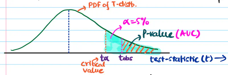
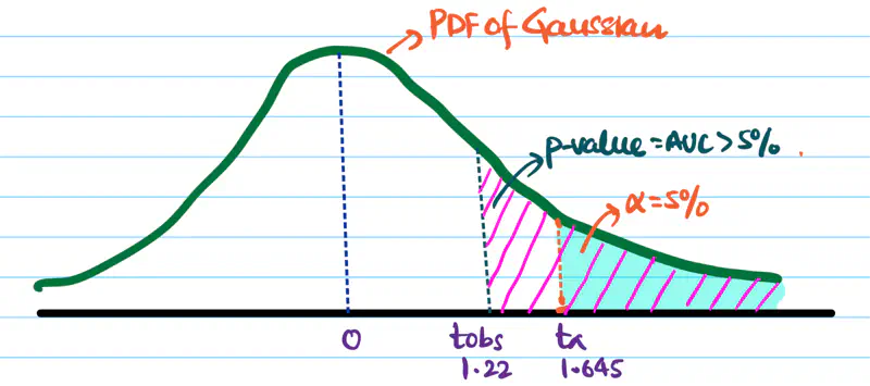
P-Value:
p-value = area under curve = probability of observing test statistic \( \ge t_{obs} \) if the null hypothesis is true.
Step 6: Accept or reject the null hypothesis, based on the significance level (\(\alpha\)).
If \(p_{value} < \alpha\), we reject the null hypothesis and accept the alternative hypothesis and vice versa.
Note: In the above example \(p_{value} < \alpha\), so we reject the null hypothesis.
We need to do a left or right sided test, or a 2-sided test, this depends upon our alternate hypothesis and test statistic.
Let’s continue our 2 sample mean T-test to understand the concept:
Left Sided/Tailed Test:
\(H_a\): Mean recovery time of medicine 1 < medicine 2, i.e, \(m_{m_1} < m_{m_2}\)
=> \(m_{m_1} - m_{m_2} < 0\)
Since, the denominator in above equation is always positive.
=> \(t_{obs} < 0\)
Therefore, we need to do a left sided/tailed test.
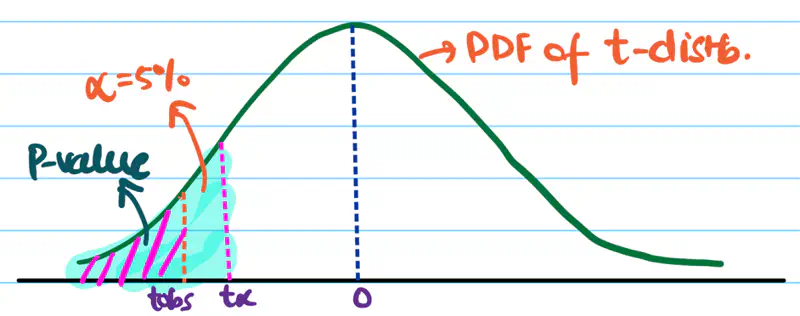
So, we want \(t_{obs}\) to be very negative to confidently conclude that alternate hypothesis is true.
Right Sided/Tailed Test:
\(H_a\): Mean recovery time of medicine 1 > medicine 2, i.e, \(m_{m_1} > m_{m_2}\)
=> \(m_{m_1} - m_{m_2} > 0\)
Similarly, here we need to do a right sided/tailed test.
2 Sided/Tailed Test:
\(H_a\): Mean recovery time of medicine 1 ⍯ medicine 2, i.e, \(m_{m_1} ⍯ ~ m_{m_2}\)
=> \(m_{m_1} - m_{m_2} < 0\) or \(m_{m_1} - m_{m_2} > 0\)
If \(H_a\) is true then \(t_{obs}\) is a large -ve value or a large +ve value.
Since, t-distribution is symmetric, we can divide the significance level \(\alpha\) into 2 equal parts.
i.e \(\alpha = 2.5\%\) on each side.
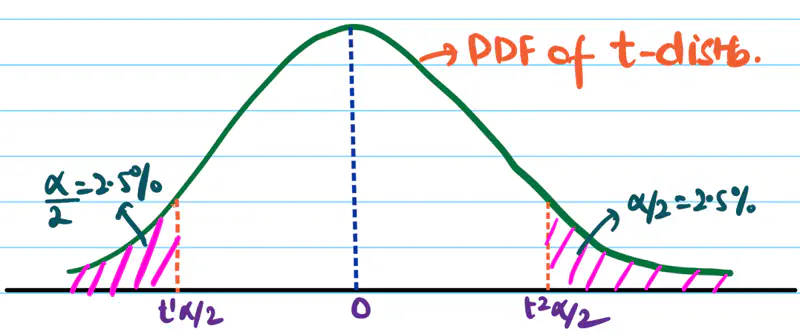
So, we want \(t_{obs}\) to be very negative or very positive to confidently conclude that the alternate hypothesis is true. We accept \(H_a\) if \(t_{obs} < t^1_{\alpha/2}\) or \(t_{obs} > t^2_{\alpha/2}\).
Note: For critical applications ‘\(\alpha\)’ can be very small i.e. 0.1% or 0.01%, e.g medicine.
It is the probability of wrongly rejecting a true null hypothesis, known as a Type I error or false +ve rate.
- Tolerance level of wrongly accepting alternate hypothesis.
- If the p-value < \(\alpha\), we reject the null hypothesis and conclude that the finding is statistically NOT so significant..
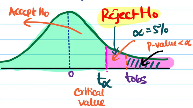
It is a specific point on the test-statistic distribution that defines the boundaries of the null hypothesis
acceptance/rejection region.
It tells us that at what value (\(t_{\alpha}\)) of test statistic will the area under curve be equal to the significance level \(\alpha\).
For a right tailed/sided test:
- if \(t_{obs} > t_{\alpha} => p_{value} < \alpha\); therefore, reject null hypothesis.
- if \(t_{obs} < t_{\alpha} => p_{value} \ge \alpha\); therefore, failed to reject null hypothesis.
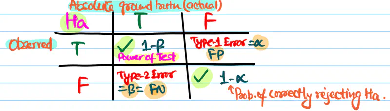
It is the probability that a hypothesis test will correctly reject a false null hypothesis (\(H_{0}\)) when the alternative hypothesis (\(H_{a}\)) is true.
Power of test = \(1 - \beta\)
Probability of correctly accepting alternate hypothesis (\(H_{a}\))
\(\alpha\): Probability of wrongly accepting alternate hypothesis \(H_{a}\)
\(\beta\): Probability of wrongly rejecting alternate hypothesis \(H_{a}\)
Yes, having a large sample size makes a hypothesis test more powerful.
- As n increases, sample mean \(\bar{x}\) approaches the population mean \(\mu\).
- Also, as n increases, t-distribution approaches normal distribution.
It is a standardized objective measure that complements p-value by clarifying whether a statistically significant
finding has any real world relevance.
It quantifies the magnitude of relationship between two variables.
- Larger effect size => more impactful effect.
- Standardized (mean centered + variance scaled) measure allows us to compare the imporance of effect across various studies or groups, even with different sample sizes.
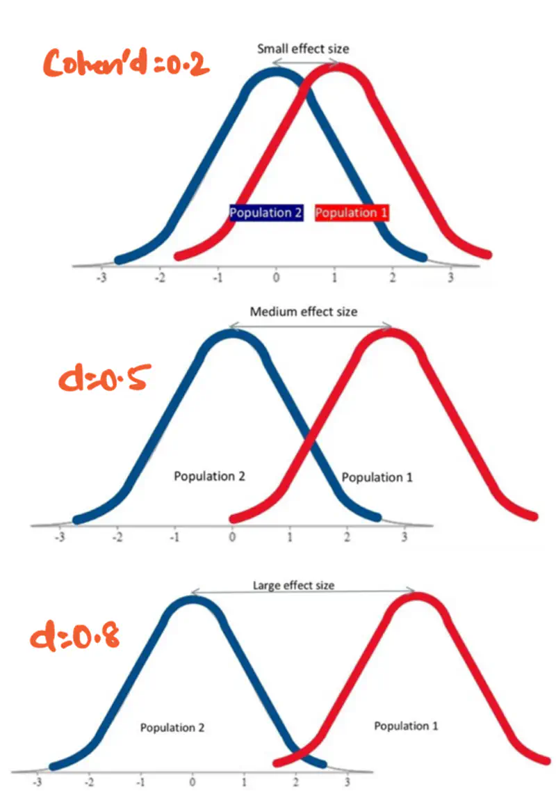
Effect size is measured using Cohen’s d formula:
\(\bar{X}\): Sample mean
\(s_p\): Pooled Standard deviation
\(n\): Sample size
\(s\): Standard deviation
Note: Theoretically, Cohen’s d value can range from negative infinity to positive infinity.
but for practical purposes, we use the following value:
small effect (\(d=0.2\)), medium effect (\(d=0.5\)), and large effect (\(d\ge 0.8\)).
More overlap => less effect i.e low Cohen’s d value.
- A study on drug trials finds that patients taking a new drug had statistically significant
improvement (p-value<0.05), compared to a placebo group.
- Small effect size: Cohen’s d = 0.1 => drug had minimal effect.
- Large effect size: Cohen’s d = 0.8 => drug produced substantial improvement.
End of Section
6 - T-Test
It is a statistical test that is used to determine whether the sample mean is equal to a hypothesized value or
is there a significant difference between the sample means of 2 groups.
- It is a parametric test, since it assumes data to be approximately normally distributed.
- Appropriate when:
- sample size n < 30.
- population standard deviation \(\sigma\) is unknown.
- It is based on Student’s t-distribution.
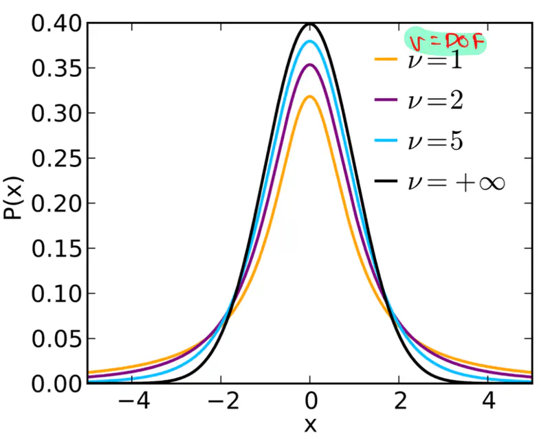
It is a continuous probability distribution that is a symmetrical, bell-shaped curve similar
to the normal distribution but with heavier tails.
Shape of the curve or mass in tail is controlled by degrees of freedom.
There are 3 types of T-Test:
- 1-Sample T-Test: Test if sample mean differs from hypothesized value.
- 2-Sample T-Test: Test whether there is a significant difference between the means of two independent groups.
- Paired T-Test: Test whether 2 related samples differ, e.g., before and after.
Generally speaking, it represents the number of independent values that are free to vary in a dataset when estimating a parameter.
e.g.: If we have k observations and their sum = 50.
The sum of (k-1) terms can be anything, but the kth term is fixed at 50 - (sum of other (k-1) terms).
So, we have only (k-1) terms that can change independently, therefore, the DOF(\(\nu\)) = k-1.
It is used to test whether the sample mean is equal to a known/hypothesized value.
Test statistic (t):
where,
\(\bar{x}\): sample mean
\(\mu\): hypothesized value
\(s\): sample standard deviation
\(n\): sample size
\(\nu = n-1 \): degrees of freedom
Tester ran the test 20 times and found the average API repsonse time to be 115 ms, with a standard deviation of 25 ms.
Is the developer’s claim valid?
Let’s verify developer’s claim using the tester’s test results using 1 sample t-test.
Null hypothesis: \(H_0\) = The average API response time is 100 ms, i.e, \(\bar{x} = \mu\).
Alternative hypothesis: \(H_a\) = The average API response time > 100 ms, i.e, \(\bar{x} > \mu\) => right tailed test.
Hypothesized mean \(\mu\) = 100 ms
Sample mean \(\bar{x}\) = 115 ms
Sample standard deviation \(s\) = 25 ms
Sample size \(n\) = 20
Degrees of freedom \(\nu\) = 19
\( t_{obs} = \frac{\bar{x} - \mu}{s/\sqrt{n}}\) = \(\frac{115 - 100}{25/\sqrt{20}}\)
= \(\frac{15\sqrt{20}}{25} = \frac{3\sqrt{20}}{5} \approx 2.68\)
Let significance level \(\alpha\) = 5% =0.05.
Critical value \(t_{0.05}\) = 1.729
Important: Find the value of \(t_{\alpha}\) in T-table
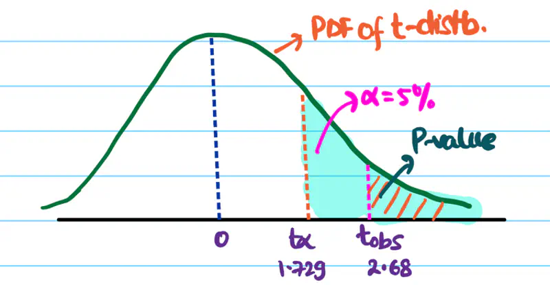
Since \(t_{obs}\) > \(t_{0.05}\), we reject the null hypothesis.
And, accept the alternative hypothesis that the API response time is significantly > 100 ms.
Hence, the developer’s claim is NOT valid.
It is used to determine whether there is a significant difference between the means of two independent groups.
There are 2 types of 2-sample t-test:
- Unequal Variance
- Equal Variance
Unequal Variance:
In this case, the variance of 2 independent groups is not equal.
Also called, Welch’s t-test.
Test statistic (t):
Equal Variance:
In this case, both samples come from equal or approximately equal variance.
Test statistic (t):
Here, degrees of freedom (for equal variance) \(\nu\) = \(n_1 + n_2 - 2\).
\(\bar{x}\): sample mean
\(s\): sample standard deviation
\(n\): sample size
\(\nu\): degrees of freedom
The AI team wants to validate whether the new ML model accuracy is better than the existing model’s accuracy.
Below is the data for the existing model and the new model.
| New Model (A) | Existing Model (B) | |
|---|---|---|
| Sample size (n) | 24 | 18 |
| Sample mean (\(\bar{x}\)) | 91% | 88% |
| Sample std. dev. (s) | 4% | 3% |
Given that the variance of accuracy scores of new and existing models are almost same.
Now, let’s follow our hypothesis testing framework.
Null hypothesis: \(H_0\): The accuracy of new model is same as the accuracy of existing model.
Alternative hypothesis: \(H_a\): The new model’s accuracy is better/greater than the existing model’s accuracy => right tailed test
Let’s solve this using 2 sample T-Test, since the sample size n < 30.
Since the variance of 2 sample are almost equal then we can use the pooled variance method.
Next let’s compute the test statistic, under null hypothesis.
DOF \(\nu\) = \(24+18-2\) = 42 - 2 = 40
Let significance level \(\alpha\) = 5% =0.05.
Critical value \(t_{0.05}\) = 1.684
Important: Find the value of \(t_{\alpha}\) in T-table
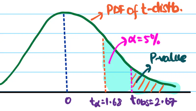
Since \(t_{obs}\) > \(t_{0.05}\), we reject the null hypothesis.
And, accept the alternative hypothesis that the new model has better accuracy than the existing model.
End of Section
7 - Z-Test
It is a statistical test used to determine whether there is a significant difference between mean of 2 groups or sample and population mean.
- It is a parametric test, since it assumes data to be normally distributed.
- Appropriate when:
- sample size \(n \ge 30\).
- population standard deviation \(\sigma \) is known.
- It is based on Gaussian/normal distribution.
- It compares the difference between means relative to standard error, i.e, standard deviation of sampling distribution of sample mean.
There are 2 types of Z-Test:
- 1-Sample Z-Test: Used to compare the mean of a sample mean with a population mean.
- 2-Sample Z-Test: Used to compare the sample means of 2 independent samples.
It is a standardized score that measures how many standard deviations a particular data point is away from the population mean \(\mu\).
- Transform a normal distribution \(\mathcal{N}(\mu, \sigma^2)\) to a standard normal distribution \(Z \sim \mathcal{N}(0, 1)\).
- Standardized score helps us compare values from different normal distributions.
Z-score is calculated as:
\[Z = \frac{x - \mu}{\sigma}\]x: data point
\(\mu\): population mean
\(\sigma\): population standard deviation
e.g:
- Z-score of 1.5 => data point is 1.5 standard deviations above the mean.
- Z-score of -2.0 => data point is 2.0 standard deviations below the mean.
Z-score helps to define probability areas:
- 68% of the data points fall within \(\pm 1 \sigma\).
- 95% of the data points fall within \(\pm 2 \sigma\).
- 99.7% of the data points fall within \(\pm 3 \sigma\).
Note:
- Z-Test applies the concept of Z-score to sample mean rather than a single data point.
It is used to test whether the sample mean \(\bar{x}\) is significantly different from a known population mean \(\mu\).
Test Statistic:
\(\bar{x}\): sample mean
\(\mu\): hypothesized population mean
\(\sigma\): population standard deviation
\(n\): sample size
\(\sigma / \sqrt{n}\): standard error of mean
Read more about Standard Error
Note: Test statistic Z follows a standard normal distribution \(Z \sim \mathcal{N}(0, 1)\).
It is used to test whether the sample means \(\bar{x_1}\) and \(\bar{x_2}\) of 2 independent samples are significantly different from each other.
Test Statistic:
\(\bar{x_1}\): sample mean of first sample
\(\bar{x_2}\): sample mean of second sample
\(\sigma_1\): population standard deviation of first sample
\(\sigma_2\): population standard deviation of second sample
\(n_1\): sample size of first sample
\(n_2\): sample size of second sample
Note: Test statistic Z follows a standard normal distribution \(Z \sim \mathcal{N}(0, 1)\).
After applying a new optimisation, and n=100 runs, yields a sample mean of 117 seconds.
Does the optimisation significantly reduce the runtime of the model?
Consider the significance level of 5%.
Null Hypothesis: \(\mu = 120\) seconds, i.e, no change.
Alternative Hypothesis: \(\mu < 120\) seconds => left tailed test.
We will use 1-sample Z-Test to test the hypothesis.
Test Statistic:
Since, significance level \(\alpha\) = 5% =0.05.
Critical value \(Z_{0.05}\) = -1.645
Important: Find the value of \(Z_{\alpha}\) in Z-Score Table
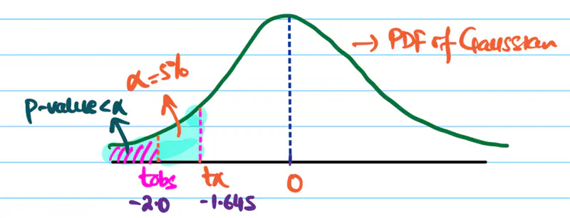
Our \(t_{obs}\) is much more extreme than the the critical value \(Z_{0.05}\), => p-value < 5%.
Hence, we reject the null hypothesis.
Therefore, there is a statistically significant evidence that the new optimisation reduces the runtime of the model.
It is a statistical hypothesis test used to determine if there is a significant difference between the proportion
of a characteristic in two independent samples or to compare a sample proportion to a known population value
- It is used when dealing with categorical data, such as, success/failure, male/female, yes/no etc.
It is of 2 types:
- 1-Sample Z-Test of Proportion: Used to test whether the observed proportion in a sample differs from hypothesized proportion.
- 2-Sample Z-Test of Proportion: Used to compare whether the 2 independent samples differ in their proportions.
The categorical data,i.e success/failure, is discrete that can be modeled as Bernoulli distribution.
Let’s understand how this Bernoulli random variable can be approximated as a Gaussian distribution for a very large sample size,
using Central Limit Theorem.
Read more about Central Limit Theorem
Note:We will not prove the complete thing, but we will understand the concept in enough depth for clarity.
\(Y \sim Bernoulli(p)\)
\(X \sim Binomial(n,p)\)
E[X] = mean = np
Var[X] = variance = np(1-p)
X = total number of successes
p = true probability of success
n = number of trials
Proportion of Success in sample = Sample Proportion = \(\hat{p} = \frac{X}{n}\)
e.g.: If n=100 people were surveyed, and 40 said yes, then \(\hat{p} = \frac{40}{100} = 0.4\)
By Central Limit Theorem, we can state that for very large ’n’ Binomial distribution’s mean and variance can be used as an
approximation for Gaussian/Normal distribution:
Since, \(\hat{p} = \frac{X}{n}\)
We can say that:
Mean = \(\mu_{\hat{p}} = p\) = True proportion of success in the entire population
Standard Error = \(SE_{\hat{p}} = \sqrt{Var[\frac{X}{n}]} = \sqrt{\frac{p(1-p)}{n}}\) = Standard Deviation of the sample proportion
Note: Large Sample Condition - Approximation is only valid when the expected number of successes and failures are both > 10 (sometimes 5).
\(np \ge 10 ~and~ n(1-p) \ge 10\)
It is used to test whether the observed proportion in a sample differs from hypothesized proportion.
\(\hat{p} = \frac{X}{n}\): Proportion of success observed in a sample
\(p_0\): Specific propotion value under the null hypothesis
\(SE_0\): Standard error of sample proportion under the null hypothesis
Z-Statistic: Measures how many standard errors is the observed sample proportion \(\hat{p}\) away from \(p_0\)
Test Statistic:
It is used to compare whether the 2 independent samples differ in their proportions.
- Standard test used in A/B testing.
A company wants to compare its 2 different website designs A & B.
Below is the table that shows the data:
| Design | # of visitors(n) | # of signups(x) | conversion rate(\(\hat{p} = \frac{x}{n}\)) |
|---|---|---|---|
| A | 1000 | 80 | 0.08 |
| B | 1200 | 114 | 0.095 |
Is the design B better, i.e, design B increases conversion rate or proportion of visitors who sign up?
Consider the significance level of 5%.
Null Hypothesis: \(\hat{p_A} = \hat{p_B}\), i.e, no difference in conversion rates of 2 designs A & B.
Alternative Hypothesis: \(\hat{p_B} > \hat{p_A}\) i.e conversion rate of B > A => right tailed test.
Check large sample condition for both samples A & B.
\(n\hat{p_A} = 80 > 10 ~and~ n(1-\hat{p_A}) = 920 > 10\)
Similarly, we can show for B too.
Pooled proportion:
\[ \bar{p} = \frac{x_A+x_B}{n_A+n_B} = \frac{80+114}{1000+1200} = \frac{194}{2200} \\[10pt] => \bar{p}\approx 0.0882 \]Standard Error(Pooled):
\[ SE=\sqrt{\bar{p}(1-\bar{p})(\frac{1}{n_1} +\frac{1}{n_2})} \\[10pt] = \sqrt{0.0882(1-0.0882)(\frac{1}{1000} +\frac{1}{1200})} \\[10pt] => SE \approx 0.0123 \]Test Statistic(Z):
\[ t_{obs} = \frac{\hat{p_B}-\hat{p_A}}{SE_{\hat{p_A}-\hat{p_B}}} \\[10pt] = \frac{0.095-0.0882}{0.0123} \\[10pt] => t_{obs} \approx 1.22 \]Significance level \(\alpha\) = 5% =0.05.
Critical value \(Z_{0.05}\) = 1.645
Since, \(t_{obs} < Z_{0.05}\) => p-value > 5%.
Hence, we fail to reject the null hypothesis.
Therefore, the observed conversion rate of design B is due to random chance; thus, B is not a better design.
End of Section
8 - Chi-Square Test
A random variable Q is said to follow a chi-square distribution with ’n’ degrees of freedom,i.e \(\chi^2(n)\),
if it is the sum of squares of ’n’ independent random variables that follow a standard normal distribution, i.e, \(N(0,1)\).
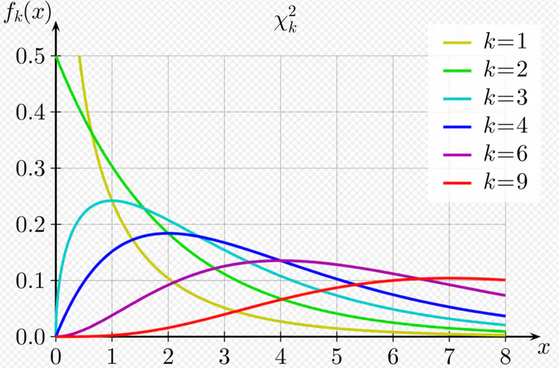
Key Properties:
- Non-negative, since sum of squares.
- Asymmetric, right skewed.
- Shape depends on the degrees of freedom; as \(\nu\) increases, the distribution becomes more symmetric and approaches a normal distribution.
Generally speaking, it represents the number of independent values that are free to vary in a dataset when estimating a parameter.
e.g.: If we have k observations and their sum = 50.
The sum of (k-1) terms can be anything, but the kth term is fixed at 50 - (sum of other (k-1) terms).
So, we have only (k-1) terms that can change independently, therefore, the DOF(\(\nu\)) = k-1.
More broadly, we can also say that sum/count of independent random variables approaches a normal distribution as the sample size increases.
Since, sample mean \(\bar{x} = \frac{sum}{n} \).
Read more about Central Limit Theorem
Note: We are dealing with categorical data, where there is a count associated with each category.
In the context of categorical data, the counts \(O_i\) are governed by multinomial distribution
(a generalisation of binomial distribution).
Multinomial distribution is defined for multiple classes or categories, ‘k’, and multiple trials ’n’.
For \(i^{th}\) category:
Probability of \(i^{th}\) category = \(p_i\)
Mean = Expected count/frequency = \(E_i = np_i \)
Variance = \(Var_i = np_i(1-p_i) \)
By Central Limit Theorem, for very large n, i.e, as \(n \rightarrow \infty\), the multinomial distribution can be approximated as a normal distribution.
The multinomial distribution of count/frequency can be approximated as :
\(O_i \approx N(np_i, np_i(1-p_i))\)
Standardized count (mean centered and variance scaled):
Under Null Hypothesis:
In Pearson’s proof of the chi-square test, the statistic is divided by the expected value (\(E_{i}\)) instead of the variance (\(Var_{i}\)),
because for count data that can be modeled using a Poisson distribution
(or a multinomial distribution where cell counts are approximately Poisson for large samples),
the variance is equal to the expected value (mean).
Therefore, \(Z_i \approx (O_{i}-E_{i})/\sqrt{E_{i}}\)
Note that the denominator is \(\sqrt{E_{i}}\) NOT \(\sqrt{Var_{i}}\).
\(O_{i}\): Observed count for \(i^{th}\) category
\(E_{i}\): Expected count for \(i^{th}\) category
Important: \(E_{i}\): Expected count should be large i.e >= 5 (typically) for a good enough approximation.
It is formed by squaring the approximately standard normal counts above, and summing them up.
For \(k\) categories, the test statistic is:
Note: For very large ’n’, the Pearson’s chi-square (\(\chi^2\)) test statistic follows a chi-square (\(\chi^2\)) distribution.
It is a non-parametric test for categorical data, i.e, does NOT make any assumption about the underlying distribution of the data, such as, normally distributed with known mean and variance; only uses observed and expected count/frequencies.
Note: Requires a large sample size.
It is used to compare the observed frequency distribution of a single categorical variable to a hypothesized or expected
probability distribution.
It can be used to determine whether a sample taken from a population follows a particular distribution,
e.g., uniform, normal, etc.
Test Statistic:
\(O_{i}\): Observed count for \(i^{th}\) category
\(E_{i}\): Expected count for \(i^{th}\) category, under null hypothesis \(H_0\)
\(k\): Number of categories
\(\nu\): Degrees of freedom = k - 1- m
\(m\): Number of parameters estimated from sample data to determine the expected probability
Note: Typical m=0, since, NO parameters are estimated.
- Kolmogorov-Smirnov (KS) Test: Compares empirical CDF with theoretical CDF of distribution.
- Anderson-Darling (AD) Test: Refinement of KS Test.
- Shapiro-Wilk (SW) Test: Specialised for normal distribution; good for small samples.
Find whether it is a fair coin (discrete uniform distribution test)?
Significance level = 5%
We need to find whether the coin is fair i.e we need to do a goodness of fit test for discrete uniform distribution.
Null Hypothesis \(H_0\): Coin is fair.
Alternative Hypothesis \(H_a\): Coin is biased towards head.
\(O_{H}\): Observed count head = 62
\(O_{T}\): Observed count head = 38
\(E_{i}\): Expected count for \(i^{th}\) category, under null hypothesis \(H_0\) = 50 i.e fair coin
\(k\): Number of categories = 2
\(\nu\): Degrees of freedom = k - 1- m = 2 - 1 - 0 = 1
Test Statistic:
Since, significance level = 5% = 0.05
Critical value = \(\chi^2(0.05,1)\) = 3.84
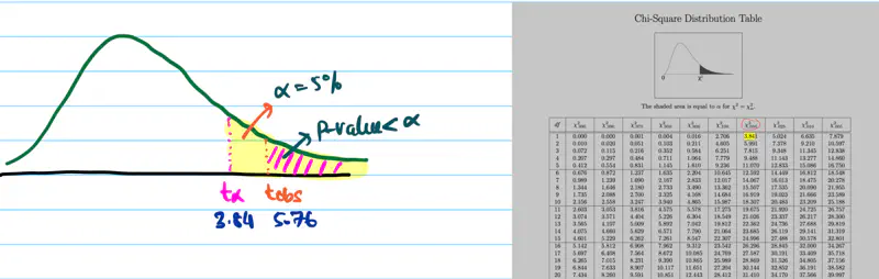
Since, \(t_{obs}\) = 5.76 > 3.84 (critical value), we reject the null hypothesis \(H_0\).
Therefore, the coin is biased towards head.
It is used to determine whether an association exists between two categorical variables,
using a contingency(dependency) table.
It is a non-parametric test, i.e, does NOT make any assumption about the underlying distribution of the data.
Test Statistic:
\(O_{ij}\): Observed count for \(cell_{i,j}\)
\(E_{ij}\): Expected count for \(cell_{i,j}\), under null hypothesis \(H_0\)
\(R\): Number of rows
\(C\): Number of columns
\(\nu\): Degrees of freedom = (R-1)*(C-1)
Let’s understand the above test statistic in more detail.
We know that, if 2 random variables A & B are independent, then,
\(P(A \cap B) = P(A, B) = P(A)*P(B)\)
i.e Joint Probability = Product of marginal probabilities.
Null Hypothesis \(H_0\): \(A\) and \(B\) are independent.
Alternative Hypothesis \(H_a\): \(A\) and \(B\) are dependent or associated.
N = Sample size
\(P(A_i) \approx \frac{Row ~~ Total_i}{N}\)
\(P(B_j) \approx \frac{Col ~~ Total_j}{N}\)
\(E_{ij}\) : Expected count for \(cell_{i,j}\) = \( N*P(A_i)*P(B_j)\)
=> \(E_{ij}\) = \(N*\frac{Row ~~ Total_i}{N}*\frac{Col ~~ Total_j}{N}\)
=> \(E_{ij}\) = \(\frac{Row ~~ Total_i * Col ~~ Total_j}{N}\)
\(O_{ij}\): Observed count for \(cell_{i,j}\)
A survey of 100 students was conducted to understand whether there is any relation between gender and beverage preference.
Below is the table that shows the number of students who prefer each beverage.
| Gender | Tea | Coffee | |
|---|---|---|---|
| Male | 20 | 30 | 50 |
| Female | 10 | 40 | 50 |
| 30 | 70 |
Significance level = 5%
Null Hypothesis \(H_0\): Gender and beverage preference are independent.
Alternative Hypothesis \(H_a\): Gender and beverage preference are dependent.
We know that Expected count for cell(i,j) = \(E_{ij}\) = \(\frac{Row ~~ Total_i * Col ~~ Total_j}{N}\)
\(E_{11} = \frac{50*30}{100} = 15\)
\(E_{12} = \frac{50*70}{100} = 35\)
\(E_{21} = \frac{50*30}{100} = 15\)
\(E_{22} = \frac{50*70}{100} = 35\)
Test Statistic:
Degrees of freedom = (R-1)(C-1) = (2-1)(2-1) = 1
Since, significance level = 5% = 0.05
Critical value = \(\chi^2(0.05,1)\) = 3.84
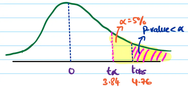
Since, \(t_{obs}\) = 4.76 > 3.84 (critical value), we reject the null hypothesis \(H_0\).
Therefore, the gender and beverage preference are dependent.
End of Section
9 - Performance Metrics
E.g.: For regression models, we have - MSE, RMSE, MAE, R^2 metric, etc.
Here, we will discuss various performance metrics for classification models.
It is a table that summarizes model’s predictions against the actual class labels, detailing where the model
succeeded and where it failed.
It is used for binary or multi-class classification problems.
| Predicted Positive | Predicted Negative | |
|---|---|---|
| Actual Positive | True Positive (TP) | False Negative (FN) |
| Actual Negative | False Positive (FP) | True Negative (TN) |
Type-1 Error:
It is the number of false positives.
e.g.: Model predicted that a patient has diabetes, but the patient actually does NOT have diabetes; “false alarm”.
Type-2 Error:
It is the number of false negatives.
e.g.: Model predicted that a patient does NOT have diabetes, but the patient actually has diabetes; “a miss”.
Many metrics are derived from the confusion matrix.
Precision:
It answers the question: “Of all the instances that the model predicted as positive, how many were actually positive?”
It measures exactness or quality of the positive predictions.
Recall:
It answers the question: “Of all the actual positive instances, how many did the model correctly identify?”
It measures completeness or coverage of the positive predictions.
F1 Score:
It is the harmonic mean of precision and recall.
It is used when we need a balance between precision and recall; also helpful when we have imbalanced data.
Harmonic mean penalizes extreme values more heavily, encouraging both metrics to be high.
| Precision | Recall | F1 Score | Mean |
|---|---|---|---|
| 0.5 | 0.5 | 0.50 | 0.5 |
| 0.7 | 0.3 | 0.42 | 0.5 |
| 0.9 | 0.1 | 0.18 | 0.5 |
Trade-Off:
Precision Focus:: Critical when cost of false positives is high.
e.g: Identify a potential terrorist.
A false positive, i.e, wrongly flagging an innocent person as a potential terrorist is very harmful.
Recall Focus:: Critical when cost of false negatives is high.
e.g.: Medical diagnosis of a serious disease.
A false negative, i.e, falsely missing a serious disease can cost someone’s life.
Analyze the performance of an access control system. Below is the data for 1000 access attempts.
| Predicted Authorised Access | Predicted Unauthorised Access | |
|---|---|---|
| Actual Authorised Access | 90 (TP) | 10 (FN) |
| Actual Unauthorised Access | 1 (FP) | 899 (TN) |
When the system allows access, it is correct 98.9% of the time.
The system caught 90% of all authorized accesses.
It is a graphical plot that shows the discriminating ability of a binary classifier system, as its
discrimination threshold is varied.
Y-axis: True Positive Rate (TPR), Recall, Sensitivity
\(TPR = \frac{TP}{TP + FN}\)
X-axis: False Positive Rate (FPR); (1 - Specificity)
\(FPR = \frac{FP}{FP + TN}\)
Note: A binary classifier model outputs a probability score between 0 and 1.
and a threshold (default=0.5) is applied to the probability score to get the final class label.
\(p \ge 0.5\) => Positive Class
\(p < 0.5\) => Negative Class
Algorithm:
- Sort the data by the probability score in descending order.
- Set each probability score as the threshold for classification and calculate the TPR and FPR for each threshold.
- Plot each pair of (TPR, FPR) for all ’n’ data points to get the final ROC curve.
e.g.:
| Patient_Id | True Label \(y_i\) | Predicted Probability Score \(\hat{y_i}\) |
|---|---|---|
| 1 | 1 | 0.95 |
| 2 | 0 | 0.85 |
| 3 | 1 | 0.72 |
| 4 | 1 | 0.63 |
| 5 | 0 | 0.59 |
| 6 | 1 | 0.45 |
| 7 | 1 | 0.37 |
| 8 | 0 | 0.20 |
| 9 | 0 | 0.12 |
| 10 | 0 | 0.05 |
Set the threshold \(\tau_1\) = 0.95, calculate \({TPR}_1, {FPR}_1\)
Set the threshold \(\tau_2\) = 0.85, calculate \({TPR}_2, {FPR}_2\)
Set the threshold \(\tau_3\) = 0.72, calculate \({TPR}_3, {FPR}_3\)
…
…
Set the threshold \(\tau_n\) = 0.05, calculate \({TPR}_n, {FPR}_n\)
Now, we have ’n’ pairs of (TPR, FPR) for all ’n’ data points.
Plot the points on a graph to get the final ROC curve.
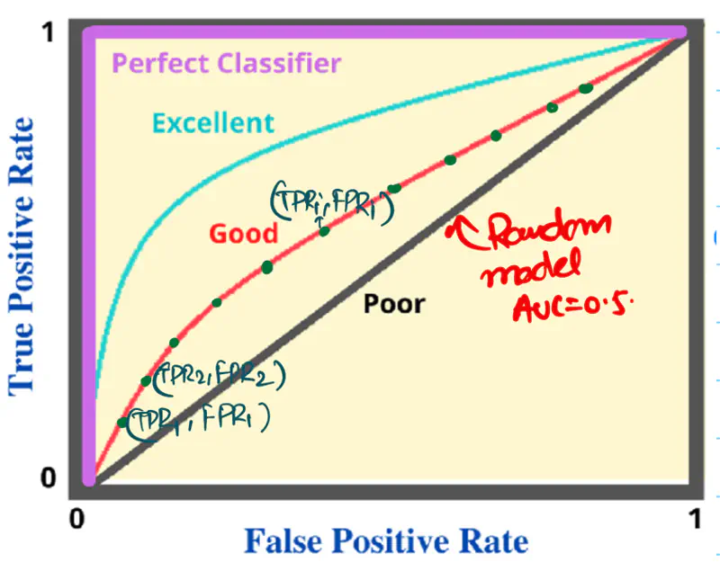
AU ROC = AUC = Area under the ROC curve = Area under the curve
Note:
- If AUC < 0.5, then invert the labels of the classes.
- ROC does NOT perform well on imbalanced data.
- Either balance the data or
- Use Precision-Recall curve.
Since, labels are randomly generated as 0/1 for binary classification, so 50% labels from each class.
Because random number generators generate numbers uniformly in the given range.
Let’s understand this with the below fraud detection example.
Below is a dataset from a fraud detection system for N = 10,000 transactions.
Fraud = 100, NOT fraud = 9900
| Predicted Fraud | Predicted NOT Fraud | |
|---|---|---|
| Actual Fraud | 80 (TP) | 20 (FN) |
| Actual NOT Fraud | 220 (FP) | 9680 (TN) |
If we check the location of above (TPR, FPR) pair on the ROC curve, then we can see that it is
very close to the top-left corner.
This means that the model is very good at detecting fraudulent transactions, but that is NOT the case.
This is happening because of the imbalanced data, i.e, count of NOT fraud transactions is 99 times
of fraudulent transactions.
Let’s look at the Precision value:
We can see that the model has poor precision,i.e, only 26.7% of flagged transactions are actual frauds.
Unacceptable precision for a good fraud detection system.
It is used to evaluate the performance of a binary classifier model across various thresholds.
It is similar to the ROC curve, but it uses Precision instead of TPR on the Y-axis.
Plots Precision (Y-axis) against Recall (X-axis) for different classification thresholds.
Note: It is useful when the data is imbalanced.
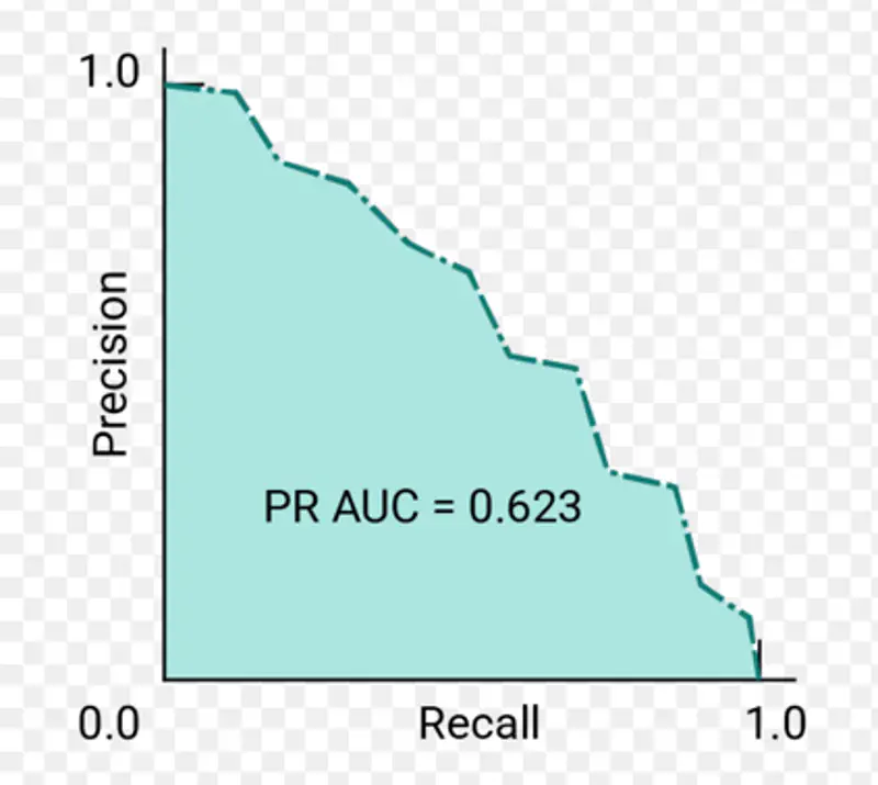
AU PRC = PR AUC = Area under Precision-Recall curve
Let’s revisit the fraud detection example discussed above to understand the utility of PR curve.
| Predicted Fraud | Predicted NOT Fraud | |
|---|---|---|
| Actual Fraud | 80 (TP) | 20 (FN) |
| Actual NOT Fraud | 220 (FP) | 9680 (TN) |
If we check the location of above (Precision, Recall) point on PRC curve, we will find that it is located near the
bottom right corner, i.e, the model performance is poor.
End of Section