This is the multi-page printable view of this section. Click here to print.
Natural Language Processing
- 1: Introduction
- 2: Text Pre-Processing
- 3: Tokenization
- 4: Text Embedding
- 5: RNN
- 6: LSTM
- 7: GRU
- 8: Attention
- 9: Self Attention
- 10: Transformer
- 11: LLM
- 12: BERT
1 - Introduction
Natural Language Processing (NLP) is a subfield of artificial intelligence that enables computers to
understand, interpret, and generate human language.
e.g. Question Answering, Summary, Dialogue Generation (Chatbot), Sentiment Analysis, Spam Classification etc.
❌ Human language is ambiguous; meaning of the sentence is determined by its context.
- He sat by the bank.
- ‘bank’ may mean a river or a financial institution.
- I saw the man with the telescope.
- the man was with a telescope, or
- he saw a man using a telescope.
- The chicken is ready to eat.
- chicken(dead) is cooked and ready to eat, or
- the chicken(alive) is hungry and ready to eat.
💡 Therefore, in NLP, it’s very important to capture the context, so that the exact meaning of the words in the sentence is understood.
Before we dive into how do we capture the context, we need to convert the human language into a form that is understandable by machines.
We know that deep learning models take vectors/matrices as input, which are collections of numbers.
So, first we need to convert the words into vectors for training the models.
First, we start with a large corpus of text required to train the model.
Corpus = large collection of text, i.e, internet scale data, such as, wikipedia, books, webpages, discussion forums etc.
Then we process the text, i.e, break down sentences into words/tokens and get their vector representations,
so that these vectors (also called word embeddings) can be used as input to train the deep learning model.
Below are the steps:
- Text Pre-Processing
- Punctuation Removal, Stop Word Removal, Lowercasing, Stemming, Lemmatization
- Tokenization
- Byte Pair Encoding, WordPiece, SentencePiece
- Text Representation (Embedding)
- OHE, BoW, TFIDF, Word2Vec, GloVe, FastText
✅ Once, we have the word embeddings now we can use them to train models that understand sentences (sequence modelling).
Let’s have a look a brief history of NLP models developed for understanding sentences:
- N-Gram (1951), Claude Shannon
- Predict the next word based on previous ’n-1’ words.
- RNN (1986), Rumelhart, Hinton, & Williams
- Predict the next word in the sequence using all the past words in the sentence (hidden state).
- LSTM (1997), Hochreiter & Schmidhuber
- Introduced long term memory, along with short term memory (as in RNN) and gates to control them.
- GRU (2014), Cho et al.
- Simplified LSTM architecture with fewer gates.
- Attention (2014), Bahdanau, Cho, & Bengio
- In machine translation instead of having a fixed context from encoder, decoder decides parts of the source sentence to pay attention, i.e, context changes for each word.
- Self Attention (2017), Vaswani et al.
- Every word in a sentence looks at every other word (including itself) to decide which word is most relevant to its own meaning in that specific context.
- Transformers (2017), Vaswani et al.
- Landmark paper that replaced sequential RNN/LSTM based models completely with Self Attention, making it highly parallelizable.
- LLM (GPT) (2018), Radford et al. (OpenAI)
- First transformer based (decoder only) architecture that led to the birth of LLMs.
- SFT, RLHF (2022), Ouyang et al. (InstructGPT)
- Fine-tuning approaches to make the LLMs useful, i.e, question answering, code generation, instruction following etc.
- BERT (2018), Devlin et al. (Google)
- Transformer based (encoder only) architecture that captures the context of a word from both sides (left & right), making it useful for natural language inference tasks.
2 - Text Pre-Processing
❌ Raw text is messy and inconsistent.
e.g., “WOw!!! The new iphone 18 pro is SOOO good! I luvv it… best phone ever? Check it out at someCoolSite.com #tech #apple”
So, first we need to do some pre-processing of this messy text, before it can be used for model training.
There are 2 main steps:
- Cleaning: Removing punctuation, lowercasing, stop word removal and stripping special characters.
- Stemming/Lemmatization: Reducing words to their root form.
Removing punctuation, lowercasing, stop word removal and stripping special characters.
- Input: “👋 Hello, together we will learn NLP (Natural Language Processing)!!!”:
- Output: “hello learn nlp natural language processing”
Reduce words to their root form, by chopping off suffixes, often resulting in non-dictionary roots; very fast.
- Input: “Running was considered better than going to gym.”
- Porter Stemmer Output: [“run", “wa”, “consid”, “better”, “than”, “go”, “to”, “gym”]
Reduce words to their root form, i.e, dictionary base form (lemma).
- Input: “Running was considered better than going to gym.
- WordNet Lemmatizer Output: [“run", “be”, “consider”, “good”, “than”, “go”, “to”, “gym”]
When to use Lemmatization or Stemming:
- ✅ Lemmatization: Accuracy; e.g., chatbots
- ✅ Stemming: Speed; e.g., searching massive datasets
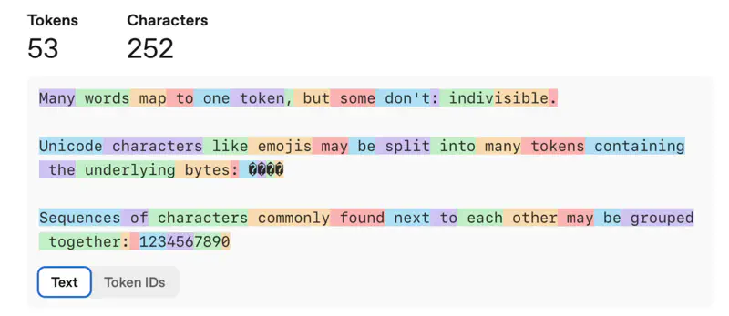
3 - Tokenization
Text is split by whitespace or punctuation.
Each unique word gets its own ‘ID’ in the vocabulary.
e.g., “The player is playing”, becomes:
[“The”, “player”, “is”, “playing”]
Issues
- Out-Of-Vocabulary (OOV): If the model has seen only “player” in the training set and at runtime it sees “players” or “playful”, then it marks them as
(Unknown). - Vocabulary Explosion: If we use full words then vocabulary size.
- No Shared Meaning: The model treats “running” and “run” as completely unrelated symbols, even though they share the same root.
Text is split into individual letters or symbols.
e.g., “Apple”, becomes:
[“A”, “p”, “p”, “l”, “e”]
Issues
- Loss of Semantics: Individual characters like “a” or “p” carry no inherent meaning.
- The model has to work much harder to learn that the sequence “A-p-p-l-e” represents a fruit.
- Long Sequences: A single sentence becomes a massive string of tokens.
- Computationally Expensive: Longer sequences require more memory and processing power to calculate relationships between tokens.
A fixed-size vocabulary that can represent any word by breaking it into meaningful sub-units.
e.g., “unhappiness”, becomes:
[“un”, “happi”, “ness”]
Benefits
- Small vocabulary size.
- No OOV (everything decomposable).
- Better generalization.
Comparison: Word-Level, Character-Level & Sub-Word Tokenization
| Feature | Word-Level | Char-Level | Sub-Word |
|---|---|---|---|
| Vocab Size | Very Large | Small | Medium (Fixed) |
| OOV Problem | Severe | None | None |
| Meaning (Per Token) | High | Low | High (Morpheme-based) |
| Sequence Length | Small | Very High | Balanced |
Originally a data compression algorithm, Byte Pair Encoding (BPE) was adapted for NLP to iteratively merge the most frequent adjacent pairs of characters into new tokens.
BPE Algorithm
- Initialization: Prepare a corpus and define a target vocabulary size ‘’. Break every word into individual characters (plus a special end-of-word symbol ).
- Frequency Count: Count all adjacent pairs of symbols in the corpus.
- Merge: Identify the pair  with the highest frequency and merge them into a single new symbol .
- Repeat: Update the corpus with the new symbol and repeat until the vocabulary reaches size ‘’ or no more merges are possible.
Example
--- Initial Word Corpus ---
Word                  Count
------------------  -------
l o w </w>                5
l o w e r </w>            2
n e w e s t </w>          6
w i d e s t </w>          3
h i g h e s t </w>        2

 Iteration 0
| Token   |   Frequency |
|---------+-------------|
| e       |          19 |
| </w>    |          18 |
| w       |          16 |
| s       |          11 |
| t       |          11 |
| l       |           7 |
| o       |           7 |
| n       |           6 |
| i       |           5 |
| h       |           4 |
Action: Merge ('e', 's')

Iteration 1
| Token   |   Frequency |
|---------+-------------|
| </w>    |          18 |
| w       |          16 |
| es      |          11 |
| t       |          11 |
| e       |           8 |
| l       |           7 |
| o       |           7 |
| n       |           6 |
| i       |           5 |
| h       |           4 |
Action: Merge ('es', 't')

Iteration 2
| Token   |   Frequency |
|---------+-------------|
| </w>    |          18 |
| w       |          16 |
| est     |          11 |
| e       |           8 |
| l       |           7 |
| o       |           7 |
| n       |           6 |
| i       |           5 |
| h       |           4 |
| d       |           3 |
Action: Merge ('est', '</w>')

Iteration 3
| Token   |   Frequency |
|---------+-------------|
| w       |          16 |
| est</w> |          11 |
| e       |           8 |
| </w>    |           7 |
| l       |           7 |
| o       |           7 |
| n       |           6 |
| i       |           5 |
| h       |           4 |
| d       |           3 |
Action: Merge ('l', 'o')

Iteration 4
| Token   |   Frequency |
|---------+-------------|
| w       |          16 |
| est</w> |          11 |
| e       |           8 |
| </w>    |           7 |
| lo      |           7 |
| n       |           6 |
| i       |           5 |
| h       |           4 |
| d       |           3 |
| g       |           2 |
Action: Merge ('lo', 'w')

Iteration 5
| Token   |   Frequency |
|---------+-------------|
| est</w> |          11 |
| w       |           9 |
| e       |           8 |
| </w>    |           7 |
| low     |           7 |
| n       |           6 |
| i       |           5 |
| h       |           4 |
| d       |           3 |
| g       |           2 |

OOV Handling Example
Original OOV: 'lowest'
BPE Segmented: ['low', 'est</w>']
OpenAI Tokenizer
WordPiece merges the pair that maximizes the likelihood of the training data.
It chooses the pair\((s_1, s_2)\) that maximizes:
- \(P(s_1, s_2)\): probability of the pair appearing together.
- \(P(s_1)P(s_2)\): probability of the pair appearing independently.
e.g: Is “unfriendly” in vocabulary? No;
Is “un” + “##friend” + “##ly” available? Yes.
where, “##” means continuation of the previous token.
Note: WordPiece is used in BERT.
SentencePiece is not just a new algorithm but a subword regularization framework that treats the input as a raw stream of characters, including spaces.
Key Innovations:
- Space as a Symbol:
- It treats whitespace as a normal character (represented as “underscore”).
- This makes it “lossless”; you can reconstruct the exact original string from the tokens.
- Algorithm Agnostic:
- It can implement both BPE and Unigram Language Model (a probabilistic approach that removes tokens that least impact the overall likelihood of the corpus).
- No Pre-tokenization:
- Unlike BPE/WordPiece, which often require a preliminary step to split text by whitespace, SentencePiece works directly on raw Unicode strings.
- This is vital for languages like Chinese or Japanese that do not use spaces between words.
4 - Text Embedding
Process of converting raw text into numerical vectors that machines can understand.
We will discuss the following ways to represent(embeddings) text as vectors:
- One Hot Encoding (OHE) (discrete)
- Bag of Words (BoW), TF-IDF (statistical)
- Word2Vec, GloVe, FastText (distributed)
Requirements of Good Text Representation(Embeddings)
- Capture meaning/similarity (semantics)
- Capture context
- Compact
Every word in the vocabulary ‘V’ is assigned a unique index.
e.g.
\[ \mathbf{v_{aardvark}} = \begin{pmatrix} 1 \\ 0 \\ 0 \\ \vdots \\ 0 \end{pmatrix}, \mathbf{v_{abacus}} = \begin{pmatrix} 0 \\ 1 \\ 0 \\ \vdots \\ 0 \end{pmatrix}, \dots , \mathbf{v_{zyzzyva}} = \begin{pmatrix} 0 \\ 0 \\ 0 \\ \vdots \\ 1 \end{pmatrix} \]Limitations
- High dimensional (curse of dimensionality)
- Sparse vectors
- No semantics is captured
- e.g., “love” vs “like” → completely different vectors
Represents a document by the frequency of words within it, disregarding grammar and word order.
Given a sequence of words in a document, \(D: <(w_1, w_2, \dots , w_T>\).
Vocabulary, \(\mathbf{v}_D = \sum_{i=1}^T \mathbf{v}_{w_i}\)
e.g. Document, D = “We learn NLP. For NLP we need to learn BoW."
- Vocabulary = [“We”, “Learn”, “NLP”, “For”, “Need”, “To”, “BOW”]
- Vector = [ 2, 2, 2, 1, 1, 1, 1]
Limitations
- Stop Word Problem: Common words like “the” or “is” appear frequently but carry little information, often drowning out the meaningful terms.
- Sparse Vector.
- Semantics not captured.
- Word ordering is not captured.
- e.g. \( \mathbf{v_{\text{man kills lion}}} = \begin{pmatrix} 0 \\ \vdots \\ 1 \\ 0 \\ \vdots \\ 1 \\ 0 \\ \vdots \\ 0 \\ 1 \\ \vdots \\ \end{pmatrix} = \mathbf{v_{\text{lion kills man}}} \)
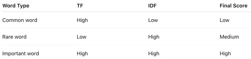
To solve the stop-word problem, TF-IDF penalizes words that appear across almost all documents.
- Term Frequency (TF): Measures how frequently a term ‘t’ occurs in a document ‘d’.
- \(TF(t, d) = \frac{\text{Number of times } t \text{ appears in } d}{\text{Total number of words in } d}\)
- Inverse Document Frequency (IDF): Measures how important a term is across the entire corpus ‘D’.
- \(IDF(t, D) = \log\left(\frac{\text{Total number of documents } N}{\text{Number of documents containing term } t}\right)\)
- \(TF-IDF(t, d, D) = TF(t, d) \times IDF (t, D)\)
If a word appears in every document (like “the,” “is,” “data”), it isn’t a good discriminator.
Note: The log function “dampens” the effect of very high frequencies.
TF-IDF Score Meaning
- The minimum TF-IDF value is 0. This occurs when a term appears in all documents (IDF = 0) or is not present in the document at all (TF = 0).
- No fixed upper bound for unnormalized TF-IDF; Max value depends on the corpus size (\(log(\text{Number of Documents})\)) and how rarely a word appears.
Let’s understand the TF-IDF score better with a very simple example.
- Document 1: “I love coffee.”
- Document 2: “I love tea.”
- Vocabulary: {‘I’, ’love’, ‘coffee’, ’tea’}
- Output Matrix:
| I | Love | Coffee | Tea | |
|---|---|---|---|---|
| Doc 1 | 0 | 0 | 0.1 | 0 |
| Doc 2 | 0 | 0 | 0 | 0.1 |
Limitations
- Semantics not captured, e.g car ≠ vehicle.
- Word ordering is not captured.
- Sparse Vector.
- Vector size = vocabulary size;
- For a vocabulary of 50,000 words, every document is a 50,000-dimensional vector consisting mostly of zeros.
- No context awareness, e.g., “bank” (river) vs “bank” (finance).
- Corpus dependency.
- Changing corpus changes representation.
- Poor generalization.
- New/unseen words → no representation
Note: TF-IDF answers → “Which words are important in this document?” , but NOT “What does this word mean?”.
Till now, we have seen that complete semantic information of each word is mapped to exactly one dimension in the vector, such as, OHE, BoW, and TFIDF.
Wouldn’t it be better if we captured the semantic and syntactic information separately in different dimensions such that similar words have similar vectors and the representation generalizes well.
e.g. Say, a word like “Apple” is represented by a 300-dimensional vector.
- Dimension 1 might represent “fruitiness,”
- Dimension 2 “redness,” and
- Dimension 3 “technology.”
- and so on …
💡 If we are able to represent a word in multiple dimensions then we can compare words in those multiple dimensions on various aspects, such that all the similar words occur together.
Distributed Representation of Words
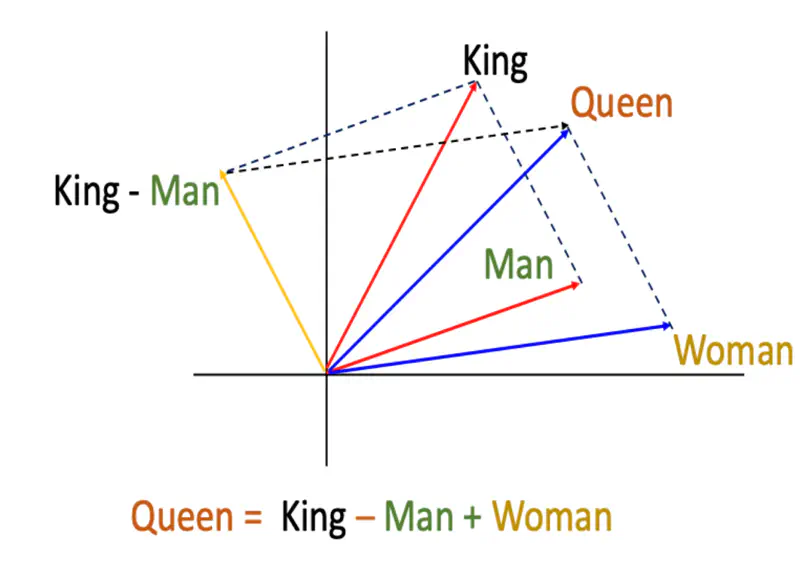
Note: We can see that similar words occur together.
“You shall know a word by the company it keeps.” ~ J.R. Firth, 1957
Word2Vec captures information about the meaning of the word based on the surrounding words, because meaning comes from context.
- Developed at Google (Mikolov et al.), 2013.
- Word2Vec moved NLP from “counting” to “predicting”.
Word2Vec uses 2 methods to learn one vector per word appearing in the corpus.
- CBOW (Continuous Bag of Words): Predicts a target word based on its context (the surrounding words).
- Best for: Smaller datasets; smooths over some noise.
- Skip-gram: Predicts the context words given a single target word.
- Best for: Large datasets; better at representing rare words.
Word2Vec Architectures
Skip-Gram predicts the surrounding context words given the center or target word.
It operates on the principle that words appearing in similar contexts tend to have similar semantic meanings, making it effective at capturing both semantic and syntactic relationships.
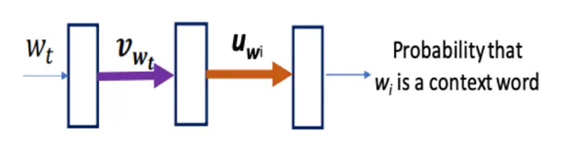
If the training example is “brown”, then the softmax output corresponding to the word “fox” will be 1, rest all units will be 0.
Note: \(\mathbf{v}_{w_t}\) is used as the final dense vector representation for the word \(w_t\).
Let’s dive deeper into Skip-Gram architecture and understand the optimization problem.
Cost Function
Problem
Here, the computation of probability of context word given center word \(P(w_{t+j} | w_t)\), and its derivative,
i.e, \(\frac{\partial {P(w_{t+j} | w_t)}}{\partial {\mathbf{v}_{w_t}}}\) (for gradient descent weight update)
is expensive if vocabulary size is large, i.e, \(|V| \gg 0\).
Note: Loss Function = Cross Entropy
Computational Scale Analysis
If our vocabulary has \(10^{5}\) words, every single update for a single word pair requires \(10^{5}\) operations.
Since a typical corpus has billions of tokens, performing \(|V|\) operations per token makes training mathematically possible but computationally intractable on standard hardware.
Solution
Negative Sampling
A clever trick !
Instead of summing over the whole vocabulary, the model only updates the “true” context word and a small sample (e.g., 5–20) of random “negative” words.
This turns a massive multiclass classification problem into a series of simple binary logistic regression problems.
- Randomly select a small number of ‘K’ non-context words for which softmax unit output is 0.
- For every “Positive” pair (words that actually appear together), we generate ‘K’ “negative” pairs (words that are randomly sampled from the dictionary and likely have no relationship).
- Positive Pair (\(w, c\)): “The quick brown fox” \(\rightarrow\)(quick, fox)
- Negative Pairs (\(w, c_{neg}\)): (quick, apple), (quick, potato), (quick, diary)
Benefit: If we have a vocabulary of 10,000 words and use , we only update weights for 6 output neurons (1 positive + 5 negative) instead of all 10,000.
Cost Function
\[log ~ \hat{P}(w_{t+j} | w_t) = \underbrace{log(\sigma(\mathbf{v}^T_{w_t}\mathbf{u}_{w_{t+j}}))}_{Positive Pair} + \sum_{k=1}^K \underbrace{log(\sigma(-\mathbf{v}^T_{w_t}\mathbf{u}_{w}))}_{Negative Pair}\]🎯 Goal is to maximize the log likelihood function.
We can see that both the terms on the left of equality is of the form \(log(\sigma(x))\), where \(x\) is the dot product \(v^Tu\).
Since, sigmoid function outputs value in the range of 0 to 1, so \(log(\sigma(x))\) range will be \((-\infty, 0]\).
Therefore, in order to maximize the value of log likelihood we need to bring it closer to 0.
Let’s see how the values of \( x, \sigma(x)\), and \(log(\sigma(x))\) vary together:
- Positive Pair: as \(x \rightarrow \infty, ~ \sigma(x) \rightarrow 1, ~ and ~ log(x) \rightarrow 0\)
- Negative Pair: as \(x \rightarrow -\infty, ~ \sigma(x) \rightarrow 0, ~ and ~ log(x) \rightarrow -\infty\)
Note: \(\sigma(-x) = 1 - \sigma(x)\)
Limitation of Word2Vec
Word2Vec only uses local context and is excellent at analogies and capturing semantics but ignores the vast amount of statistical information available in the global co-occurrence counts.
As, we saw earlier in the case of TF-IDF that uses the statistics of the entire corpus.
GloVe leverages global co-occurrence matrix, allowing it to better understand how words relate across the entire dataset, resulting in superior semantic analogies and better representation of relationships between distant words.
Research Paper: GloVe: Global Vectors for Word Representations, Pennington et al., Stanford University, 2014, https://nlp.stanford.edu/pubs/glove.pdf
Glove model leverages statistical information by training only on the nonzero elements in a word-word co-occurrence matrix, and uses matrix factorization to generate low-dimensional word representations.
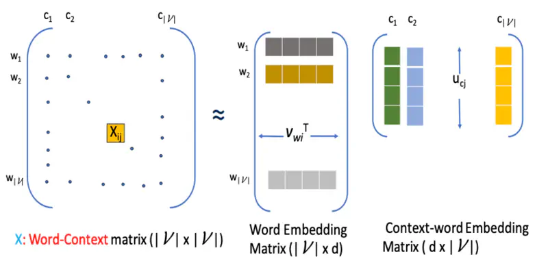
\(X_{ij}\) : Number of times word \(c_j\) appears in the context of word \(w_i\)
Word-word matrix or word-context matrix \(X\) is factorized into 2 matrices, such that:
\[X_{ij} \approxeq \mathbf{v}^T_{w_i}\mathbf{u}_{c_j} \text{ or } X_{ij} \approxeq exp(\mathbf{v}^T_{w_i}\mathbf{u}_{c_j})\]Note: We do an exponentiation because dot product can be negative but the word count is always positive.
We have to find the 2 matrices such that the difference between the dot product and the actual word co-occurrence count is minimum.
This can be formulated as an optimization problem, because we have to find some kind of optimum, in this case minimum value.
Optimization Problem
\[ \underset{\mathbf{v}_w, \mathbf{u}_c}{\mathrm{min}} \lVert \mathbf{V}_w \mathbf{U}_c - \text{log}(\mathbf{X}) \rVert^2_F \]where, F is Frobenius Norm
Read more about Optimization
Read more about Frobenius Norm
Estimate word and context vectors by solving the optimization problem:
\[ \underset{\mathbf{v}_w, \mathbf{u}_c, b, \tilde{b}}{\mathrm{min}} \sum_{i,j=1}^{|V|} f(X_{ij}) ~ ( \mathbf{v}^T_{w_i}\mathbf{u}_{c_j} + b_i + \tilde{b}_j - \text{log}(X_{ij}))^2\]\[f(x) = \begin{cases} (x/x_{max})^{\alpha} & \text{if } x < x_{max} \\ 1 & otherwise \end{cases} \]Note: In the paper they empirically found that the most suitable value of \(\alpha = 3/4\).
Let’s understand all the parameters.
- \(f(X_{ij})\): Weighting function.
- If \(X_{ij} = 0\): \(f(x) = 0\); Ignore pairs that never co-occur.
- If \(X_{ij}\) is small: \(f(x)\) is also small, but increases as count increases.
- If \(X_{ij}\) is very large (for stop words): \(f(x)\) saturates (usually at 1); prevents common stop-words from over-influencing the vectors.
- Bias terms
- \(b_i\): Captures the “inherent frequency” of the target word \(w_i\).
- If word \(w_i\) is very common (like “the”), \(b_i\) will be large.
- \(\tilde{b}_j\): Captures the “inherent frequency” of the context word \(c_j\).
- \(b_i\): Captures the “inherent frequency” of the target word \(w_i\).
- ✅ GloVe can often outperform Word2Vec on smaller datasets because it extracts more statistical signal from every available word pair.
- ✅ Pre-trained Word2Vec models are often significantly larger (e.g., 3.4GB for Google News) compared to GloVe’s more lightweight variants (e.g., 150MB for Wiki-Gigaword), making GloVe better for resource-constrained applications.
- ✅ In practice, we start with GloVe for its stability and availability of pre-trained vectors, then experiment with Word2Vec if the specific syntactic nuances of their dataset are not being captured.
Instead of treating each word as an atomic unit, FastText breaks words into a “bag” of character ’n-grams’ (skip-gram), which allows it to capture morphological information and effectively handle rare or out-of-vocabulary (OOV) words.
- Developed by Facebook AI Research (FAIR).
e.g. if n = 3, (typically, n = 3, 4, 5, 6):
<where> : { <wh, whe, her, ere, re>, <where>}
Note: FastText also uses Skip-Gram architecture, similar to Word2Vec, wo we will not discuss skip gram model and dive in directly into understanding the difference between FastText and Word2Vec approaches.
Word2Vec (skip-gram model)
\[log ~ P(w_{t+j} | w_t) = \mathbf{v}^T_{w_t}\mathbf{u}_{w_{t+j}} - log\sum_{w \in V} \mathbf{v}^T_{w_t}\mathbf{u}_{w}\]FastText (skip-gram model)
Represent a word by the sum of the vector representations of its character n-grams and the word itself:
- \(G_w\): : set of all n−grams appearing in word ‘w’; (typically n = 3,4,5,6)
- \(z_w^g\): vector associated with n-gram \(g \in G_w\)
- \(\mathbf{v}_{w} = \sum_{g \in G_{w}} z_{w}^g\)
FastText Skip-Gram Example

- ✅ Use Word2Vec if we have a massive, clean English dataset and need fast, high-quality syntactic vectors for common words.
- ✅ Use GloVe if your primary goal is finding thematic similarities (e.g., “doctor” to “hospital”) across very large documents.
- ✅ Use FastText if you are dealing with non-English languages, social media text, or any application where new words appear frequently.
5 - RNN
N-gram model is a probabilistic tool used to predict the next item in such a sequence by looking at the previous \(n-1\) items.
The “n” in n-gram refers to the number of items in the sequence.
- Unigram (\(n=1\)): Single words (e.g., “We”, “learn”, “RNN”).
- Bigram (\(n=2\)): Pairs of consecutive words (e.g., “We learn”, “learn RNN”).
- Trigram (\(n=3\)): Triplets of consecutive words (e.g., “We learn RNN”)
Limitation
Natural language text may not be of fixed size.
Every sentence is of different length.
We cannot use n-gram model, because it calculates the probability of a word based on the ‘\(n-1\)’ preceding words, relying only on a fixed, finite context window.
So, we need a model that can process an input of any length and use all the sequence information from the past.
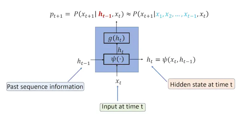
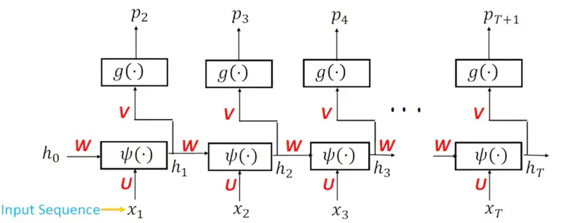
At each step, the RNN maintains a “hidden state” that captures information about the words seen so far.
Recurrent Relation
\[P(x_{t+1} | x_1, x_2, \dots, x_t) \approx P(x_{t+1} | h_{t-1}, x_t)\]\(h_{t-1}\): Hidden/latent vector that captures all the information seen till time instance ‘\(t-1\)’.
Note: Hidden state can theoretically capture information from the entire history of the sequence.
RNN Architecture
RNN Parameters
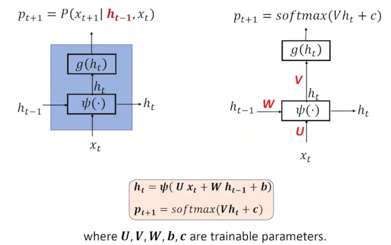
Note: Number of parameters is independent of input sequence length, because the same neural network is processing different words at different time stamps.
Sequence Information
See below how different words are input at different time stamps and the hidden state stores the sequence information seen till that time stamp.
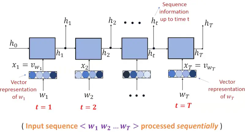
Note: The input \(x_1, x_2, \dots, x_T \) are the vector representations of the words or word embeddings, earlier OHE was used, but after 2013, Word2Vec or GloVe etc. are mostly used.
Teacher Forcing
Say we are training the RNN model for text generation or language modeling,
i.e, we predict the next word based on all the words seen in the past.
e.g. Let’s assume that we are using the following sentence to train the model:
“This is a cat.”
Now at time ’t’ the model sees the current word (\(w_t\)) “a” and tries to predict the “t+1” or next word.
It generates a probability distribution (softmax output) \(p_{t+1}\) of all the words in the vocabulary.
But the model has just started training, and it has no idea of sentences now, so it can predict any garbage value,
which may be totally meaningless.
So, in order to train the model and learn the patterns from the training data instead of feeding the predicted word \(p_{t+1}\)
as the next input i.e \(w_{t+1}\), we feed the actual word i.e “cat” as \(w_{t+1}\).
This is called Teacher Forcing.
Note: This stops the error (caused by predicting some garbage value during training) from being propagated through the network.
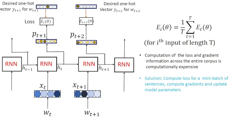
RNN Algorithm
- For every sentence ‘i’ in the corpus:
- For every token ‘t’ in the sentence:
- Compute probability distribution \(p_t\) on the vocabulary, given the previous ‘t-1’ words in the sentence.
- Compute the loss (cross entropy) between \(p_t\) and \(y_t\) (desired OHE). \[ E_t(\theta) = - \sum_{j=1}^{|V|} y_{t,j} ~ \text{log}(p_{t,j}) \]
- Compute the average overall training loss for the sentence ‘i’. \[ E_i(\theta) = \frac{1}{T} \sum_{t=1}^{T} E_t(\theta) \]
- For every token ‘t’ in the sentence:
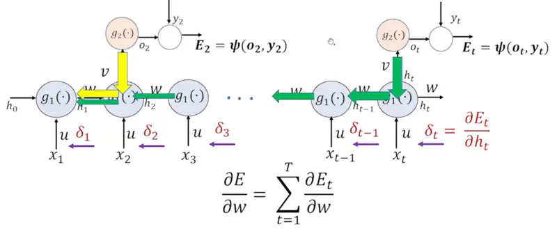
- Compute gradient information using back propagation through time and update model parameters.
Calculate the error at each time step and propagate it backward to update RNN weights.
Forward Pass
- \(a_t = Ux_t + Wh_{t-1} + b\)
- \(h_t = \sigma(a_t) = \sigma(Ux_t + Wh_{t-1} + b)\), (activation function = sigmoid, tanh, ReLU etc.)
- \(o_t = Vh_t + c\)
- \(p_{t+1} = \text{softmax} (o_t)\)
- \(E_t = \psi(o_t, y_t)\), (cross -entropy loss)
Derivative of Error wrt to weight:
\[\frac{\partial E}{\partial w } = \sum_{t=1}^T \frac{\partial E_t}{\partial w }\]We can re-write it using the chain rule of differentiation:
\[\frac{\partial E}{\partial w } = \sum_{t=1}^T \frac{\partial E_t}{\partial h_t } \frac{\partial h_t}{\partial w }\]Let, \(\delta_t = \frac{\partial E_t}{\partial h_t }\)
Similarly, error at ‘k-th’ hidden state:
\[\frac{\partial E_t}{\partial h_k } = \frac{\partial E_t}{\partial h_t }. \frac{\partial h_{t} } {\partial h_{t-1} }. \frac{\partial h_{t-1} }{\partial h_{t-2} } \dots \frac{\partial h_{k+1} } {\partial h_k }\]\[\implies \frac{\partial E_t}{\partial h_k } = \delta_t \prod_{i=k+1}^t \frac{\partial h_{i} } {\partial h_{i-1} }\]Let’s calculate \(\frac{\partial h_{t} } {\partial h_{t-1}}\) now:
\[\frac{\partial h_{t} } {\partial h_{t-1}} = \frac{\partial h_{t} } {\partial a_{t}}. \frac{\partial a_{t} } {\partial h_{t-1}}\]\[ \because h_t = \sigma(a_t)\]\[ \tag{1} \implies \frac{\partial h_{t} } {\partial a_{t}} = \sigma'(a_t) \]\[\because a_t = Ux_t + Wh_{t-1} + b\]\[ \tag{2} \implies \frac{\partial a_{t} } {\partial h_{t-1}} = W\]Therefore, combining equations 1 & 2:
\[\therefore \frac{\partial h_{t} } {\partial h_{t-1}} = \frac{\partial h_{t} } {\partial a_{t}}. \frac{\partial a_{t} } {\partial h_{t-1}} = \sigma'(a_t).W = \text{(Activation Derivative).(Weight)}\]Now, let’s revisit the error at ‘k-th’ hidden state:
\[\frac{\partial E_t}{\partial h_k } = \delta_t \prod_{i=k+1}^t \frac{\partial h_{i} } {\partial h_{i-1} }\]where, \(\delta_t = \frac{\partial E_t}{\partial h_t }\)
So, lets understand the vanishing gradient problem using an example.
Say, we have a sentence with 10 words.
- \(\lVert W \rVert = 0.7 < 1\)
- Gradient of activation function (sigmoid or tanh) = 0.2 \[\frac{\partial E_t}{\partial h_k } \propto \prod_{i=1}^{10} \text{Activation Gradient x Weight}\] \[ (0.7 \times 0.2)^{10} = (0.14)^{10} = 2.89 \times 10^{-9} \]
Therefore, the signal dies as it goes from the 10-th to first word.
The gradient value is so low that the weights will literally have no updates, hence effectively the early layers of the model stop learning.
Solution
- Skip connections
- ReLU activation (derivative 1)
Let’s continue the above vanishing gradient example, but this time with some different values to illustrate exploding gradient problem.
- \(\lVert W \rVert = 2 > 1\)
- Gradient of activation function (ReLU) = 1
Therefore, the gradients become excessively large, leading to massive, erratic updates to the model weights.
The model fails to converge, making the loss function fluctuate wildly instead of decreasing.
Solution
- Gradient clipping (need only direction of the gradient)
- L1 or L2 Regularization (forces weights to be small)
- Text Generation (One to Many)
- Sentiment Classification (Many to One)
- Machine Translation (Many to Many)
Note: The input \(x_1, x_2, \dots, x_T \) are the vector representations of the words or word embeddings, earlier OHE was used, but after 2013, Word2Vec or GloVe etc. are mostly used.
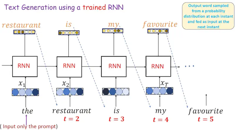
Text Generation (One to Many)
We just give one word as input to the RNN, and it keeps on generating text, by just keep predicting the next word.
Therefore, one-to-many mapping.
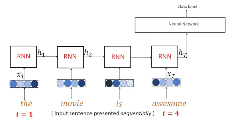
Sentiment Classification (Many to One)
We give a sentence as input for which we want the RNN to predict the sentiment as positive, negative or neutral, and we just get that one word as output.
For sentiment analysis, the RNN take the sentence as input and generates an encoded hidden state \(h_T\) for the entire sentence as output.
And this encoded vector representation of the sentence \(h_T\) is fed into another simple neural network for classification of the sentiment.
Hence, it is of the kind many-to-one mapping.
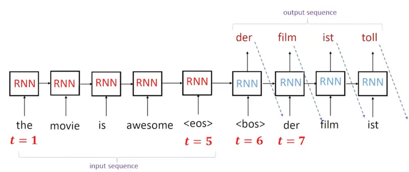
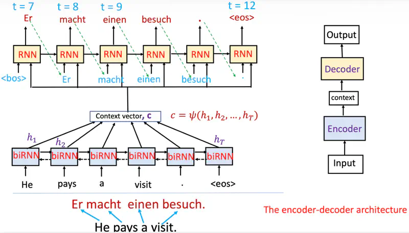
Machine Translation (Many to Many)
Machine Translation means language translation, here we use 2 RNNs, one as encoder for encoding the input language sentence,
and another RNN as decoder for generating the translated language sentence.
Hence, many-to-many mapping.
Encoder Decoder Architecture
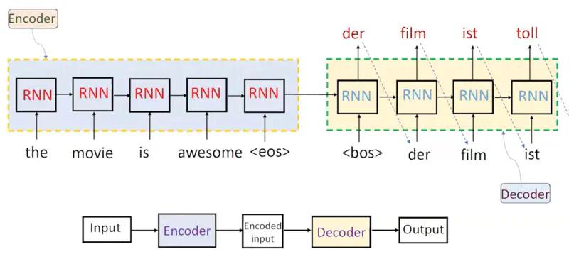
Note: The Red(encoder) and Blue(decoder) RNN blocks are different with different parameters.
- Bi-Directional RNN (Bi-RNN)
- Multi-Layer Bi-RNN
Bi-RNN
Processes sentences by analyzing it in both forward and backward directions.
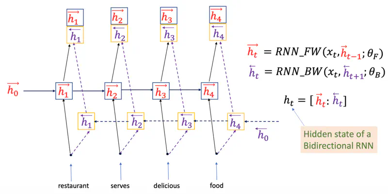
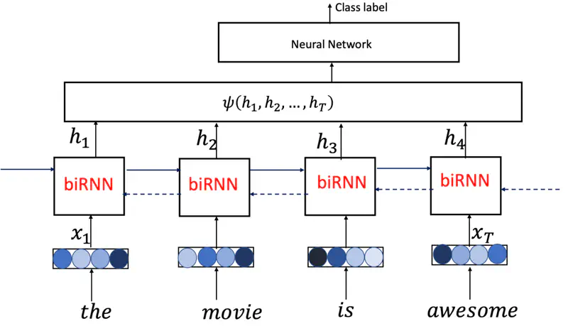
We can use Bi-RNN for sentence classification, and it will perform better than vanilla RNN, because it processes the sentence from both forward and backward direction, hence it has better and more rich context.
Sentence Classification
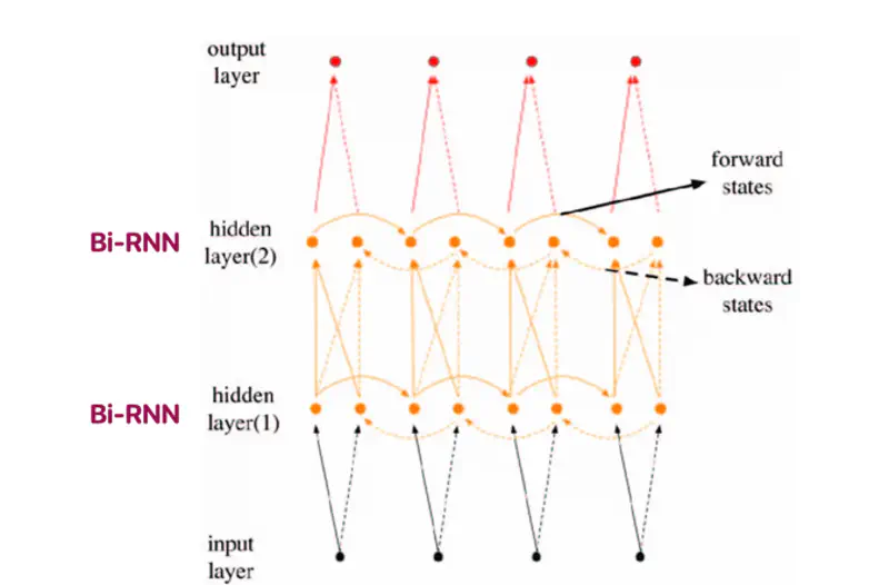
Multi Layer Bi-RNN
Stacking multiple Bi-RNN layers allows the model to learn complex patterns and high-level representations.
6 - LSTM
RNNs are not good at capturing long range dependencies (due to vanishing gradient problem).

By the time the RNN is processing “not entertaining” it forgets the subject, i.e, “Jurassic Park movie” because they are separated too far.
LSTM solves vanishing gradient problem by introducing:
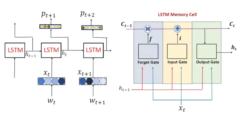
- Cell State (\(C_t\)): which acts as a “long-term” memory conveyor belt that runs parallel to the
- Hidden State (\(h_t\)): the “short-term” working memory (similar to RNN)
LSTM Memory Cell
LSTM Architecture
- Each gate in an LSTM functions as a single-layer feedforward neural network that lives inside the LSTM cell.
- Each gate has its own unique, learnable weight matrices (\(W\)) and bias vectors (\(b\)).
Decides what information from the previous cell state (\(C_{t-1}\)) is no longer useful and should be discarded.
\[f_t = \sigma(W_f \cdot [h_{t-1}, x_t] + b_f)\]- \(f_t = 0\): “forget” the previous memory entirely.
- \(f_t = 1\): “remember” everything.
Read more about Vector Operations
Read more about Activation Function
This stage decides what new information will be stored in the cell state (\(C_t\)).
- Input Gate: Decides which values to update. \[ i_t = \sigma(W_i \cdot [h_{t-1}, x_t] + b_i) \]
- Candidates: Creates a vector of new candidate values that could be added to the state. \[\tilde{C}_t = \tanh(W_C \cdot [h_{t-1}, x_t] + b_C)\]
- Update the Cell State: This is the “memory update” where the old memory is scaled by the forget gate and the new information is scaled by the input gate. \[C_t = \underbrace{f_t \odot C_{t-1}}_{\text{Filtered\ Old\ Info}} + \underbrace{i_t \odot \tilde{C}_t}_{\text{Filtered\ New\ Info}}\]
Read more about Vector Operations
Read more about Activation Function
Determines the next hidden state (\(h_t\)).
\[o_t = \sigma(W_o \cdot [h_{t-1}, x_t] + b_o) \]\[h_t = o_t \odot \tanh(C_t)\]This ‘\(h_t\)’ is used for predictions and as input for the next time step.
Read more about Vector Operations
Read more about Activation Function
- Sigmoid (Gates): Outputs 0 to 1;
- For “gating” (blocking or passing info).
- Tanh (Candidate): Outputs -1 to 1;
- Allows the candidate to either add to the memory (positive values) or subtract/correct the memory (negative values).
- Element Wise Product: \[ \mathbf{a} \odot \mathbf{b} = \begin{bmatrix} a_1 \\ a_2 \\ \vdots \\ a_n \end{bmatrix} \odot \begin{bmatrix} b_1 \\ b_2 \\ \vdots \\ b_n \end{bmatrix} = \begin{bmatrix} a_1 b_1 \\ a_2 b_2 \\ \vdots \\ a_n b_n \end{bmatrix} \]
Gates Summary
| Component | Role |
|---|---|
| Forget Gate | Decide which information to delete. |
| Input Gate | Decide which information to add. |
| Candidate | Actual new information. |
| Cell State | Long-term memory; conveyor belt. |
| Output Gate | Decide the next hidden state (short-term memory). |
Now let’s understand how back propagation through time happens in LSTM.
It is similar to RNN as LSTM is also sequential in nature and processes words in a sentence one by one.
- Cell State = \(C_t = f_t \odot C_{t-1} + i_t \odot \tilde{C}_t\)
- Gradient = \(\frac{\partial c_{t} } {\partial c_{t-1}} = f_t\)
- Recursively (for all words at different time steps): \[ \frac{\partial c_{t} } {\partial c_{k}} = \prod_{i=k+1}^t f_i\]
Therefore, in LSTM , the gradient is determined by the forget gate \(f_t\).
- If the information is important then the network sets the \(f_t = 1\).
- This means the gradient can flow backwards through hundreds of time steps without being scaled down to zero.
Note: Therefore, unlike RNNs, the vanishing/exploding gradient problem is significantly reduced in LSTM, because of the stable gradient flow, allowing LSTM to learn long range dependencies.
In RNN, the gradient is given by:
\[ \frac{\partial E_t}{\partial h_k } = \delta_t \prod_{i=k+1}^t \sigma'(a_i).W \propto \prod \text{Activation Gradient x Weight} \]Read more about Back Propagation Through Time in RNN
Read more about Vanishing Gradient Problem
First of all let us understand what is the meaning of “Carousel”.
Carousel 🎠 is a rotating circular amusement ride with seats (often horses) commonly called a merry-go-round, or a circular conveyor system.
And, now let us understand the meaning of Constant Error Carousel.
If we place a “message” (the gradient) on a horse, and the carousel rotates with no friction or resistance (\(f_t=1\)), the information keeps circulating exactly as it is for an infinite number of rotations.
In other words, if the forget get output for a word is set to 1, then the model does not forget it even if there are infinite number words before it till the beginning of the sentence, i.e, no vanishing gradient problem.
7 - GRU
LSTMs are complex, which makes them slower to train and more computationally intensive.
- three gates (forget, input, output) and many parameters.
- separate long-term memory (cell state) and short term memory (hidden state).
GRU is simplified LSTM with fewer gates, fewer parameters and simpler architecture, while retaining the ability to capture long-term dependencies, often leading to faster training times and reduced computational costs.
- Simpler Architecture:
- GRU has two gates (reset, update) instead of three.
- This reduces the number of weight matrices by roughly 25-33%, leading to faster training and lower memory consumption.
- Structural Simplicity:
- By merging the “Cell State” (\(C_t\)) and “Hidden State” (\(h_t\)) into a single vector, it eliminates the redundant storage of information.
- Performance on Small Data:
- Due to fewer parameters, GRUs are often less prone to overfitting than LSTMs when training on smaller datasets.
GRU Memory Cell
GRU Architecture
- Each gate in an GRU functions as a single-layer feedforward neural network that lives inside the GRU cell.
- Each gate has its own unique, learnable weight matrices (\(W\)) and bias vectors (\(b\)).
Decides how much of the past hidden state (\(h_{t-1}\)) is relevant to calculating the current candidate.
\[r_t = \sigma(U_r x_t + W_r h_{t-1} + b_r)\]- \(r_t = 0\): “forget” the past context entirely.
- \(r_t = 1\): use everything from the past.
Read more about Vector Operations
Read more about Activation Function
This is the “suggestion” for what the new state should look like.
\[\tilde{h}_t = \tanh(U x_t + W(r_t \odot h_{t-1}) + b_h)\]Note: If \(r_t=0\), then \(r_t \odot h_{t-1}\) will wipe out the previous state completely.
Read more about Vector Operations
Read more about Activation Function
Performs a linear interpolation (slider) between the old state and the new suggestion.
\[z_t = \sigma(U_z x_t + W_z h_{t-1} + b_z)\]Final state:
\[h_t = \underbrace{z_t \odot h_{t-1}}_{\text{Keep\ the\ Old}} + \underbrace{(1 - z_t) \odot \tilde{h}_t}_{\text{Adopt\ the\ New}} \]Read more about Vector Operations
Read more about Activation Function
- Sigmoid (Gates): Outputs 0 to 1;
- For “gating” (blocking or passing info).
- Tanh (Candidate): Outputs -1 to 1;
- Allows the candidate to either add to the memory (positive values) or subtract/correct the memory (negative values).
- Element Wise Product: \[ \mathbf{a} \odot \mathbf{b} = \begin{bmatrix} a_1 \\ a_2 \\ \vdots \\ a_n \end{bmatrix} \odot \begin{bmatrix} b_1 \\ b_2 \\ \vdots \\ b_n \end{bmatrix} = \begin{bmatrix} a_1 b_1 \\ a_2 b_2 \\ \vdots \\ a_n b_n \end{bmatrix} \]
Gates Summary
| Component | Role |
|---|---|
| Reset Gate | “Clear the cache for a new sub-topic.” |
| Candidate | Propose new state. |
| Update Gate | Mix old + new info. |
Now let’s understand how back propagation through time happens in GRU.
It is similar to LSTM as GRU is also sequential in nature and processes words in a sentence one by one.
- Hidden State = \(h_t = z_t \odot h_{t-1} + (1 - z_t) \odot \tilde{h}_t\)
- Gradient = \(\frac{\partial h_t}{\partial h_{t-1}} = z_t + (1-z_t)(W.r_t.tanh')\)
Recursively (for all words at different time steps): \[ \frac{\partial h_t}{\partial h_{k}} = \prod_{i=k+1}^t z_i + (1-z_i)(W.r_i.tanh')\]
Therefore, in GRU , the gradient is mostly determined by \(z_t\).
- If the information is important then the network sets the \(z_t = 1\).
- This means the gradient can flow backwards through hundreds of time steps without being scaled down to zero.
Note: Therefore, unlike RNNs, the vanishing/exploding gradient problem is significantly reduced in GRU, because of the stable gradient flow, allowing GRU to learn long range dependencies.
In RNN, the gradient is given by:
\[ \frac{\partial E_t}{\partial h_k } = \delta_t \prod_{i=k+1}^t \sigma'(a_i).W \propto \prod \text{Activation Gradient x Weight} \]Read more about Back Propagation Through Time in RNN
Read more about Vanishing Gradient Problem
First of all let us understand what is the meaning of “Carousel”.
Carousel 🎠 is a rotating circular amusement ride with seats (often horses) commonly called a merry-go-round, or a circular conveyor system.
And, now let us understand the meaning of Constant Error Carousel.
If we place a “message” (the gradient) on a horse, and the carousel rotates with no friction or resistance (\(f_t=1\)), the information keeps circulating exactly as it is for an infinite number of rotations.
In other words, if the forget get output for a word is set to 1, then the model does not forget it even if there are infinite number words before it till the beginning of the sentence, i.e, no vanishing gradient problem.
Let us understand how GRU works with the help of few examples.
1. Context Shift
Say, there is a context shift between sentences, i.e, say , the previous sentence discussed ‘Stars’
and in the current sentence we start discussing “Fish”.
Clearly, there is a context shift, and we want to the network to forget the previous context entirely and start fresh.
In that case \(r_t=0, ~ z_t=0 \), so that the current input ‘\(x_t\)’ is passed as it is.
2. Ignore Current Input
Say, we have a GRU processing a long review to determine sentiment:
“The phone I bought yesterday, despite having a slightly scratched screen that makes it annoying to use sometimes, is absolutely amazing and has a black charger.”
- The model reads “absolutely amazing” and updates its hidden state to a strong positive sentiment.
- Later the review adds irrelevant details like - “has a black charger”,
- so GRU learns to set \(z_t \approx 1\) when these words are processed, and ignores them.
Note: When GRU wants to ignore current input to preserve long-term memory, it sets \(z_t\) close to 1.
3. Default Behavior (RNN)
GRU isn’t trying to store long-term memories; it is simply processing the current input \(x_t\)
in the context of the immediately preceding hidden state \(h_{t-1}\).
- Reset Gate \(r_t = 1\): The candidate hidden state \(\tilde{h_{t}}\) has full access to the previous hidden state (\(h_{t-1}\)).
- Nothing from the past is blocked.
- Update Gate (\(z_t = 0\)): The network decides to entirely replace the old state with the new candidate state.
Note: GRU essentially “forgets” the past and behaves like a standard Simple RNN.
8 - Attention
Entire input (\(h_1, h_2, \dots, h_T\) ) is encoded into one fixed-length vector.
So, as the length of an input sentence increases performance of a basic encoder–decoder deteriorates rapidly,
because of vanishing gradient problem.
Read more about Vanishing Gradient Problem
Encoder-Decoder Architecture (RNN)
Decoder decides parts of the source sentence to pay attention to.
By letting the decoder have an attention mechanism, we relieve the encoder from the burden of having to
encode all information in the source sentence into a fixed-length vector.
While decoding an output pay attention to only relevant inputs.
Decoder Context
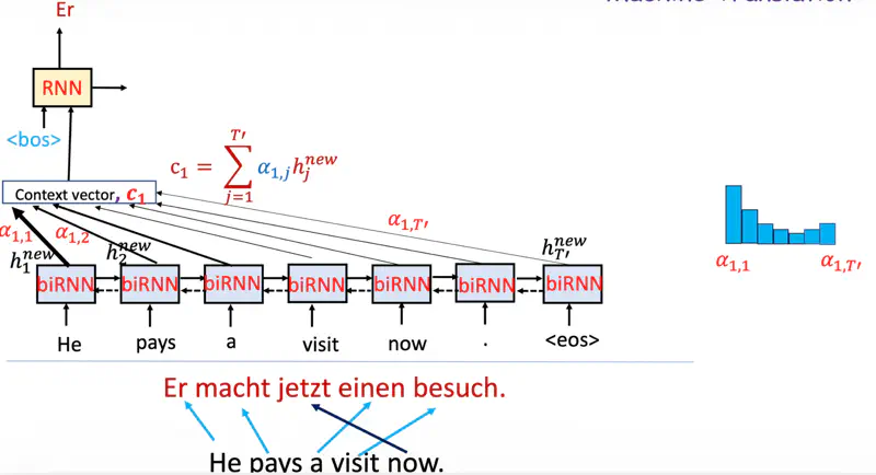
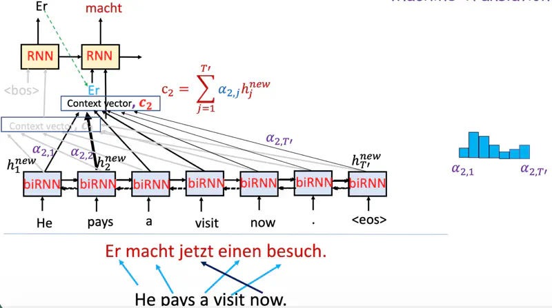
Note: Now the decoder context is not fixed.
While predicting the next word, the decoder (instead of relying only on the final encoder hidden state)
dynamically pays attention to only relevant context from encoder at that time step.
Why it matters?
This allows the decoder to “look back” at the entire input sequence, preventing the information loss that occurs
in basic encoder-decoder models when handling long sentences.
Goal
To determine the context vector (relevant) at each time step of decoder.
Before that we need to understand the meaning of few terms, viz., “Query”, “Key” & “Value”.
Research Paper: Neural Machine Translation by Jointly Learning to Align and Translate ; Dzmitry Bahdanau, Kyunghyun Cho, Yoshua Bengio, 2014, https://arxiv.org/pdf/1409.0473
In the context of Attention mechanism, Query (Q), Key (K), and Value (V) are metaphors borrowed from retrieval systems
(like a database or a search engine) to describe how information is accessed.
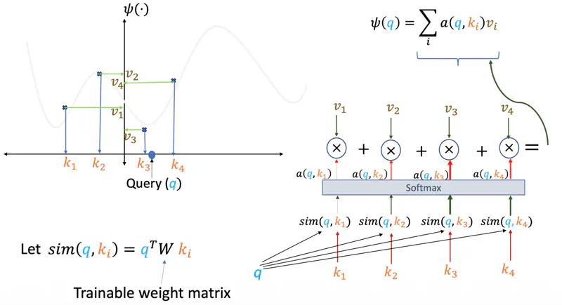
Let’s understand these terms via a “data fitting” problem.
Data Fitting
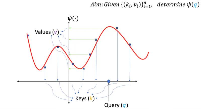
We are give some data points, i.e, some keys (\(k_i\)) and corresponding values (\(v_i\)), and the task is to find
the best fit curve (\(\psi(q)\)) so that in future if we have a new query point ‘\(q\)’ we should be able
to determine(predict) the corresponding value for the query point.
Something similar to linear regression.
Similarity Score
One of the ways can be that we find the similarity (dot product) of the query point ‘\(q\)’ with every key (\(k_i\)),
if the similarity score is high means they are closer, and vice versa, then we can take the corresponding values (\(v_i\))
scaled by the similarity score and sum them up to get the predicted value for the query point ‘\(q\)’.
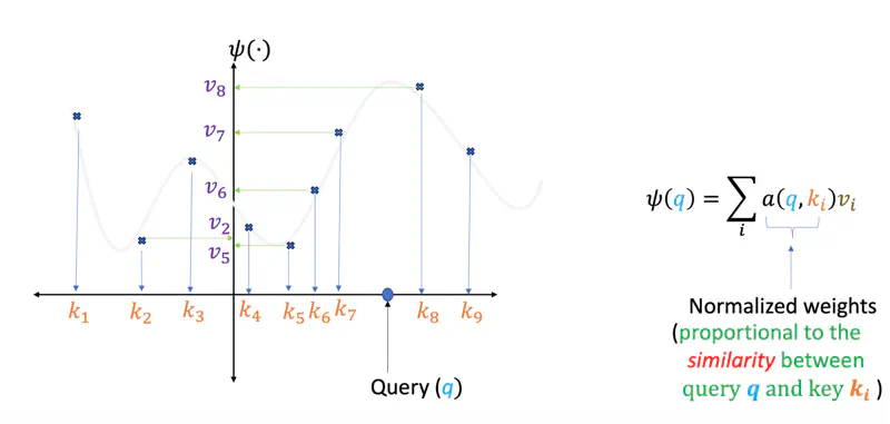
Here, in above example query point ‘\(q\)’ is closer to keys \(k_7\) and \(k_8\), hence the predicted value for the query will be more close to \(v_7\) and \(v_8\) as compared to \(v_1\) or \(v_2\), which are quite far away.
Softmax
Moreover, we can apply a softmax on the similarity scores, so that the higher scores are amplified (winner takes most),
thus giving us better prediction.
This turns our prediction into a weighted average of the values \(v_i\).

Note: Instead of a fixed curve, the model learns the best way to represent ‘\(q\)’ and ‘\(k\)’
so that the “similarity” perfectly captures the relationship we re trying to predict.
We can also have a trainable weight matrix ‘\(W\)’ whose parameters can be learnt during training.
Attention
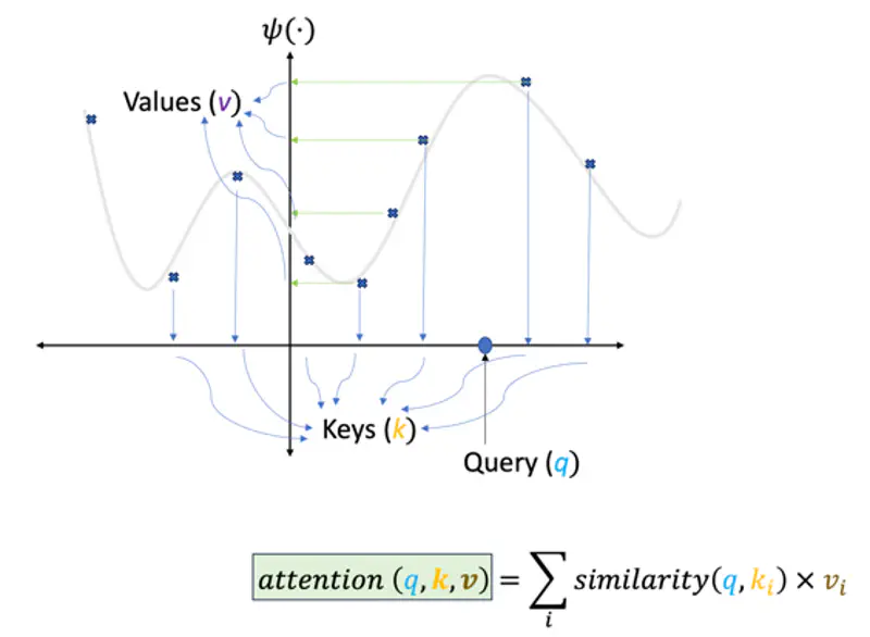
Therefore, the attention score (\(q,k,v\)) for a query ‘\(q\)’, given keys ‘\(k_i\)’ and values ‘\(v_i\)’ is the summation of all query and key similarity scores similarity(\(q, k_i\)) multiplied by their corresponding values ‘\(v_i\)’.
Bahdanau Attention was designed for the RNN based encoder-decoder architecture used for machine translation.
Encoder Decoder (Cross) Attention
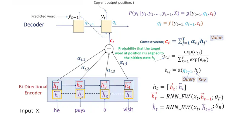
- Query: Decoder’s previous state (\(q_{t-1}\)).
- Keys: Encoder’s knowledge points from the source sentence, i.e, hidden state (\(h_j\)).
- Values: Encoder’s knowledge points from the source sentence, i.e, hidden state (\(h_j\)).
- The model “fits” the current context by calculating which source points are most relevant to the word it is currently predicting.
Let us understand all the terminologies used in the diagram above in detail:
- Alignment Function: A small neural network to see how well the Decoder’s “need” matches the Encoder’s “offer”.
- \(a(q_{t−1}, h_j) = v_a^T \tanh(W_a q_{t-1} + U_a h_j)\); Additive Attention
- Alignment Score or Energy, \(e_{tj} = a(q_{t−1}, h_j)\)
- Attention Weight: Softmax operation ; takes the raw “importance scores” (\(e_{ij}\)) and converts them into a probability distribution.
- Ensures that all \(\alpha_{ij}\)are between 0 and 1 and that they sum to 1.
- This makes the context vector (\(c_t\)) a stable weighted average.
- Softmax, \(\alpha_{tj} = \frac{\exp(e_{tj})}{\sum_{k=1}^T \exp(e_{tk})}\)
- Context Vector: Weighted sum of the encoder hidden states (the Values).
- \(c_t = \sum_{j=1}^T \alpha_{tj} h_j\)
Note: Bahdanau used additive attention, which is slow because of the addition step.
Dot Product Attention
\[a(q_{t−1}, h_j) = q_{t-1} ^T h_j\]Note: Faster to compute dot product than additive attention.
Research Paper: Effective Approaches to Attention-based Neural Machine Translation, Luong et al., 2015, https://arxiv.org/pdf/1508.04025
Scaled Dot Product Attention
\[a(q_{t−1}, h_j) = \frac{q_{t-1} ^T h_j}{\sqrt{dim(h_j)}}\]Research Paper: Attention Is All You Need, Vaswani et al. , 2017, https://arxiv.org/pdf/1706.03762
9 - Self Attention
RNNs process words sequentially, i.e, one by one.
- To understand word 20, you must first process words 1 to 19.
- By the time the model gets to the end of a long sentence, it often “forgets” the beginning (vanishing gradient problem).
Read more about Vanishing Gradient Problem

Note: Luong Attention (2015) used “dot product” based attention was faster than Bahdanau Attention (2014) (additive), but was still RNN based Seq2Seq model.
In 2017, Transformer architecture, proposed that “Self-Attention” can be used completely for machine translation instead of RNNs.
Using “Self-Attention” made the model highly parallelizable because the matrix calculations can be done on GPUs in parallel.
Transformer Architecture
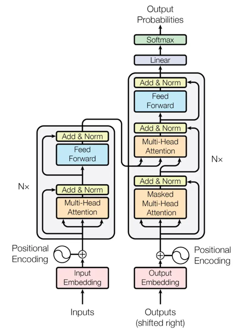
Research Paper: Attention Is All You Need, Vaswani et al. , 2017, https://arxiv.org/pdf/1706.03762
Primary reason we need self-attention is that words do not have a fixed meaning; their meaning is defined by their neighbors and context.
Example
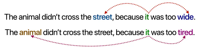
Note: Depending upon the context “it” will refer to “street” or “animal”.
Unlike older models that read left-to-right, self-attention sees the whole sentence at once, allowing it to catch relationships whether they are side-by-side or miles apart.
Every word in a sentence looks at every other word (including itself) to decide which word is most relevant to its own meaning in that specific context.
Self-Attention
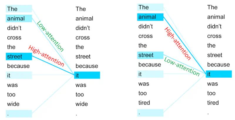
In the first sentence, “it” pays ‘high attention’ to street and ’low attention’ to animal.
And, in the second sentences, “it” pays ‘high attention’ to animal and ’low attention’ to street.
Unlike RNNs, the calculation for a token does not depend on the computation of the previous token.
All tokens can attend to all other tokens at the same time, i.e,
the attention scores (dot products between ‘\(q\)’ and ‘\(k\)’) are computed for all pairs of tokens simultaneously on GPU cores, not one-by-one.
Attention Mechanism
The attention score (\(q,k,v\)) for a query ‘\(q\)’, given keys ‘\(k_i\)’ and values ‘\(v_i\)’ is the summation of all query and key similarity scores similarity(\(q, k_i\)) multiplied by their corresponding values ‘\(v_i\)’.
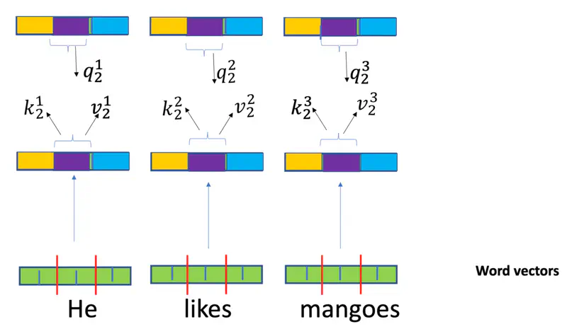
- Query (\(q_i = W_Q^T x_i\)): “What am I looking for?”
- Key (\(k_i = W_K^T x_i\)): “What do I offer?” (The label others use to find me).
- Value (\(v_i =W_V^T x_i\)): “What information do I actually carry?”
Note: \(x_i \in \mathbb{R}^{d_{model} \times 1}\)is the input word vector and \(W^Q, W^K \in \mathbb{R}^{d_{model} \times d_k} \text{ and } W^V \in \mathbb{R}^{d_{model} \times d_v}\)are learned weight matrices.
Individual Attention
The “match” between two words is calculated using a “dot product”.
If word ‘\(i\)’ wants to know how much it should care about
word ‘\(j\)’, it compares its ‘Query’ to the other word’s ‘Key’:
Self Attention Score
We pack all the individual queries, keys, and values into matrices \(Q, K, \text{ and } V\), where,
Note: ‘\(k\)’ is the dimension of \(Q, K, V\) vectors.
Self Attention Example
Why do we scale the dot product ?
\[\text{Attention}(Q, K, V) = \text{softmax}\left(\frac{QK^T}{\sqrt{d_k}}\right)V\]Research paper says that -
“We suspect that for large values of \(d_k\), the dot products grow large in magnitude,
pushing the softmax function into regions where it has extremely small gradients.
To counteract this effect, we scale the dot products by \(\frac{1}{\sqrt{d_k}}\)”
Gradient of Softmax:
\[\frac{\partial \sigma_i}{\partial z_j} = \begin{cases} \sigma_i(1 - \sigma_i) & \text{if } i = j \\ -\sigma_i\sigma_j & \text{if } i \neq j \end{cases} \]Combining both cases:
\[\frac{\partial \sigma_i}{\partial z_j} = \sigma_i (\delta_{ij} - \sigma_j)\]where, \(\delta_{ij}\) is the Kronecker delta (1 if \(i=j\) (diagonal), 0 otherwise).
e.g., say, if Softmax (\(\sigma_i\)) = 0.99,
then gradient \(\frac{\partial \sigma_i}{\partial z_j} = \sigma_i(1 - \sigma_i) = (0.99)*(0.01) = 0.0099 \)
which is a very low value, so the weight updates will effectively be negligible.
Dividing by \(\sqrt{d_k}\) reduces the variance back to 1, keeping the scores in a moderate range.
Therefore, the scaling factor \(\frac{1}{\sqrt{d_k}}\) acts as a stabilizer, preventing the model from having extreme confidence in a few places, which enables smoother training.
10 - Transformer
Transformer replaced recurrence with attention, enabling faster training and superior performance in NLP and AI tasks.
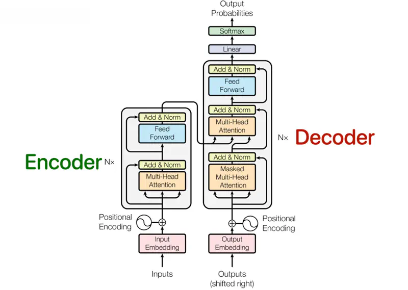
Source: Attention is all you need, Vaswani et al., 2017; https://arxiv.org/pdf/1706.03762
Transformer Architecture
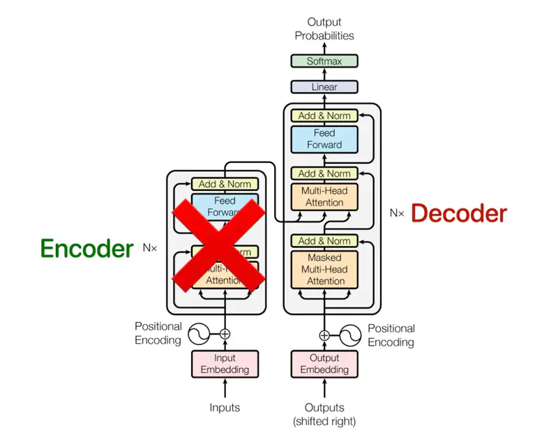
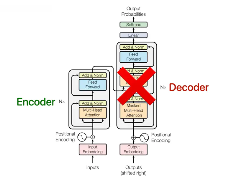
It was designed for machine translation, so it has 2 parts, viz., encoder and decoder.
Encoder
The encoder is composed of a stack of N = 6 identical layers.
- Each encoder layer has 2 sub-layers:
- Multi-Head Self Attention
- Fully connected Neural Network (Feed Forward)
- Residual connection around each of the sub-layers.
- Each sub-layer has layer normalization.
Decoder
The decoder is also composed of a stack of N = 6 identical layers.
- Each decoder layer has 3 sub-layers:
- Masked Multi-Head Attention
- Multi-Head Encoder Decoder (Cross) Attention
- Fully connected Neural Network (Feed Forward)
- Residual connection around each of the sub-layers.
- Each sub-layer has layer normalization.
Transformer replaced recurrence with attention.
3 kinds of attention are used in the transformer architecture:
- Multi-Head Self Attention (Encoder)
- Masked Multi-Head Attention (Decoder)
- Encoder Decoder (Cross) Attention (Decoder)
Unlike older models that read left-to-right, self-attention sees the whole sentence at once, allowing it to catch relationships whether they are side-by-side or miles apart.
Every word in a sentence looks at every other word (including itself) to decide which word is most relevant to its own meaning in that specific context.
We have discussed self attention in detail in the previous article.
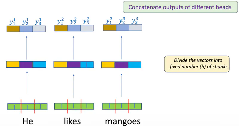
In a single-head attention system, the model has to condense all relationships into one attention score.
e.g., The Reserve Bank of India headquarters in Mumbai, sits on the bank of the Mithi River.
If a word like “bank” refers to both a “river” and “financial institution” in a complex sentence,
a single head tries to average those two different meanings.
By averaging them, we often end up with a blurry representation that does not capture either meaning well.
Allows the model to “dissect” the word.
Each head can look at different aspects of a sentence, such as, syntax (subject-verb), semantics(meaning), pronouns, etc.
- Head 1 can focus on the “river” context while
- Head 2 focuses on the “financial institution” context.
- No need to compromise (average).
- Also, each head can be processed in parallel.
Multi-Head Attention
Multi-Head
Each head is an independent attention mechanism.
Each head has its own set of learnable weight matrices (\(W_i^Q, W_i^K, W_i^V\)).
In decoder (auto-regressive), a token can only see itself and the tokens that came before it.
So, we add a mask to hide the future words.
where,\(M\): Mask (a square matrix of the same size as the attention scores).
- \(M = 0\): for positions we want to keep (“past” and “current” tokens)
- \(M = 1\): for positions we want to hide (“future” tokens).
e.g.
\[M = \begin{bmatrix} 0 & -\infty & -\infty \\ 0 & 0 & -\infty \\ 0 & 0 & 0 \end{bmatrix}\]Note: Softmax function is what actually performs the “masking” by turning those ‘\(-\infty\)’ values into zeros.
The “queries” come from the previous decoder layer, and the “keys” and “values” come from the output of the encoder.
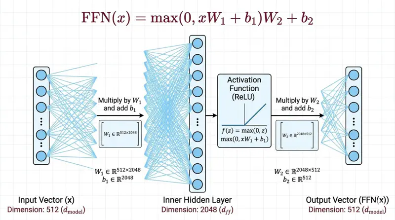
Fully connected Feed Forward Network introduces non-linear activation functions that allows the model to learn complex, non-linear relationships that attention(linear operation) alone cannot capture.
\[FFN(x) = max(0, xW_1 + b_1)W_2 + b_2 \]Feed Forward Network
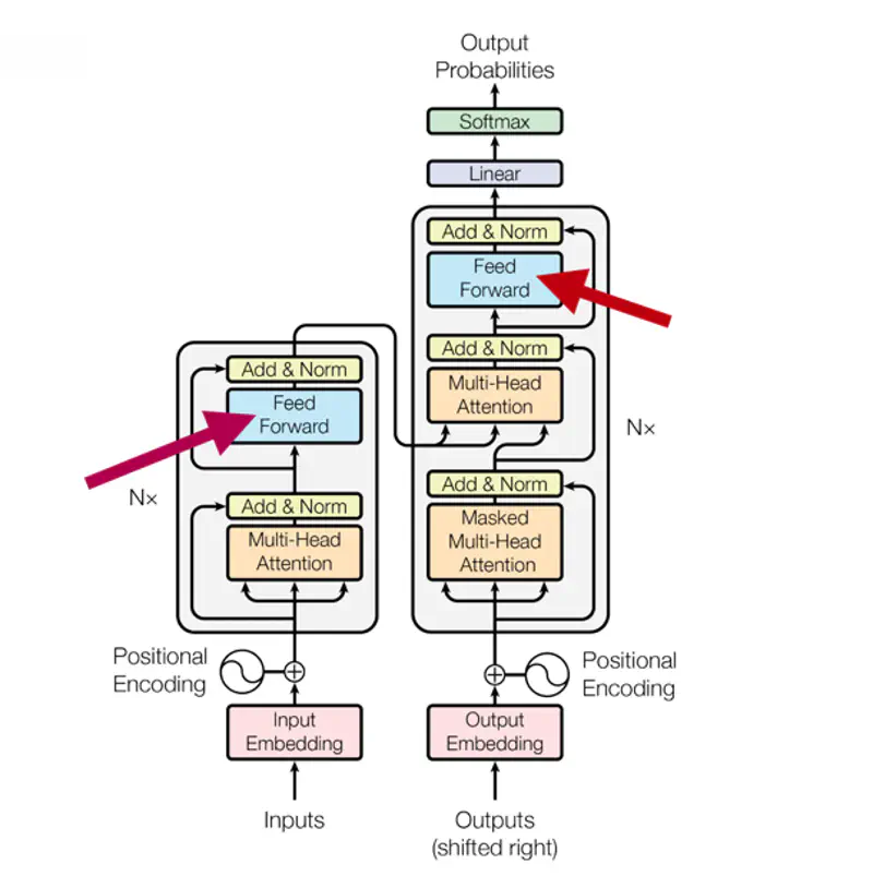
Note: The dimensionality of input and output is \(d_{model}\) = 512, and the inner-layer has dimensionality \(d_{ff}\) = 2048.
- Residual connection is used to mitigate the vanishing gradient problem.
- Skip-connections allow original input features to skip layers and be preserved, which helps the model avoid losing information in deep networks.
- But, the most vital role of residual connection is to solve the “degradation problem”.
Degradation Problem
Counter-intuitively, as model depth increases, accuracy tends to saturate and then degrade rapidly;
not because of overfitting, but because of optimization failure.
In a deep neural network (without residuals), the optimization surface becomes so rugged and chaotic that
it becomes very difficult to reach the local minima through gradient descent.
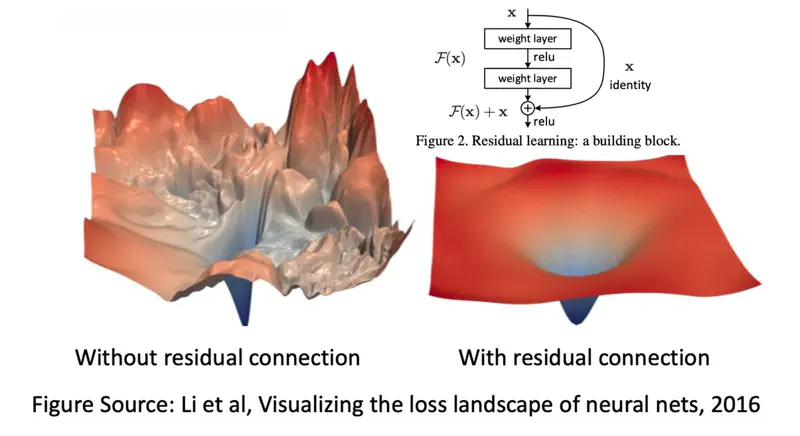
Note: A layer can simply pass the input through unchanged (identity mapping) if it does not find useful features.
Unlike Batch Normalization, which normalizes across the mini-batch for each individual feature, Layer Normalization normalizes across all the features (dimensions) for a single training instance.
- By centering mean (\(\mu\)) around zero and scaling them to variance (\(\sigma^2\)) of one, it prevents exploding or vanishing gradients, enables faster convergence.
- The mean (\(\mu\)) and variance (\(\sigma^2\)) are calculated over all features(dimensions) for that specific token.
Reason: Transformers primarily use LayerNorm because it treats each token independently.
This is critical for natural language processing (NLP) where sentences in a batch often have different lengths.
Limitations of Self Attention
Self-attention mechanism treats a sentence as a set of tokens rather than a sequence, it is inherently permutation-invariant.
e.g. “Cat eats fish.” is same as “Fish eats cat.”
Positional Encoding
So, in order to differentiate the relative position of words, Transformer architecture introduced positional encoding.
where, ‘\(pos\)’: position and ‘\(i\)’: dimension
In simple, terms each position ‘\(pos\)’ is encoded using sine and cosine functions.
This was mainly chosen to easily represent the ‘relative position’ of two words as a linear function.
Note: The formula uses \(i\) (the dimension index) to vary the frequency of the sine/cosine waves across the \(d_{model}\)-dimensional vector.
Relative Position
Say, we want to know the relative position for a word that is ‘\(k\)’ steps away.
- Position of word 1: ‘\(pos\)’ 
- Position of word 2: ‘\(pos\)’+ ‘\(k\)’
We know that:
\[\sin(A + B) = \sin(A)\cos(B) + \cos(A)\sin(B)\]\[\cos(A + B) = \cos(A)\cos(B) - \sin(A)\sin(B)\]\[\sin(pos + k) = \sin(pos)\cos(k) + \cos(pos)\sin(k)\]\[\cos(pos + k) = \cos(pos)\cos(k) - \sin(pos)\sin(k)\]So, we can represent the relative position of the second word at ‘\(pos\)’+ ‘\(k\)’, as a linear function of first word at ‘\(pos\)’.
\[\begin{bmatrix} \sin(pos + k) \\ \cos(pos + k) \end{bmatrix} = \begin{bmatrix} \cos( k) & \sin(k) \\ -\sin(k) & \cos(k) \end{bmatrix} \begin{bmatrix} \sin(pos) \\ \cos(pos) \end{bmatrix}\]All the information about Transformer architecture ends here, and the below positional encoding techniques are not a part of transformer architecture.
Just adding them here for the time being, because the concepts are related.
RoPE positional encoding is used in Llama and Mistral LLMs.
Does not add a vector to the embedding, instead, it rotates the Query (\(Q\)) and Key (\(K\)) vectors in 2D planes.
After rotation, when we take the dot product, we automatically get the relative position of tokens.
where ‘\(m\)’ is the position
Ignores the embeddings entirely and modifies the attention scores directly.
For every head, we subtract a penalty from the attention score proportional to the distance between tokens.
where ‘\(m\)’ is a head-specific slope
11 - LLM
- Generative Pre-Trained Transformer (GPT); Decoder only
- Bidirectional Encoder Representations from Transformers (BERT); Encoder only; Sentiment analysis, Question answering, Search query etc.
- Bidirectional and Auto-Regressive Transformers (BART); Encoder-Decoder; Text summarization, Document denoising (reconstruct corrupted text) etc.
- Text-To-Text Transfer Transformer (T5); Encoder-Decoder; Translation, Text summarization, etc; uses task-specific prefix
GPT Architecture (Decoder Only)
GPT (2018) was the first Large Language Model (LLM) based on Transformer (decoder only).
Because, of the highly parallelizable architecture of Transformer, it was possible to scale and train the model on
internet scale data, which gave us the magical powers of LLMs.
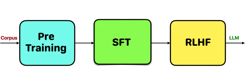
LLM is first pre-trained on vast internet scale dataset to understand the language and then it is fine-tuned to do desired tasks, such as question answering.
The LLM training is broadly divided into 3 phases:
- Pre-Training
- Supervised Fine-Tuning (SFT)
- Reinforcement Learning from Human Feedback (RLHF)
LLM Training Phases
Model is trained on a massive, unlabeled dataset (e.g., internet scale) to learn general language features, grammar, syntax, and reasoning patterns, using self-supervised learning techniques.
The self-supervised techniques are:
- Causal Language Modeling (Auto-regressive)
- Predict next token (used in GPT).
- Masked Language Modeling (used in BERT)
- A percentage of tokens in a sentence (typically 15%) are randomly hidden or “masked,” and the model must predict these missing words using context from both directions (bidirectional).
- Next Sentence Prediction
- Model is given two sentences and must determine if the second sentence naturally follows the first in the original text.
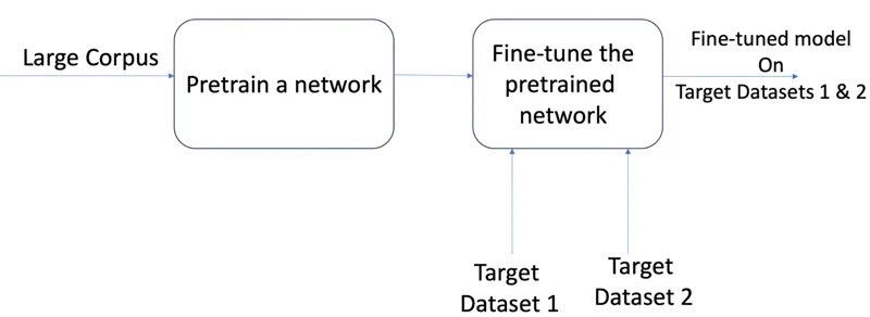
Now we can take the “pre-trained” model that has already learned general language patterns and fine tune it for different tasks.
‘Transfer learning’ is primarily used to save time and computational resources when we have a limited amount of labeled data for a specific task.
By starting with a model that already “understands” general patterns—like shapes in images or grammar in text, we can adapt it to a new, related task with much less training.
Transfer Learning
While pre-training provides a broad knowledge of syntax, SFT focuses on alignment, teaching the model to follow specific instructions and produce functional, context-aware results.
- Code Generation
- The model is trained on high-quality instruction-code pairs.
- e.g., “Prompt: Write a Python function for binary search” → “Output: [Code snippet]”.
- The model is trained on high-quality instruction-code pairs.
- Math & Reasoning (Chain of Thought)
- Instead of training the model to give the answer directly (Prompt\(\rightarrow\) Answer), we train it to generate a rationale (Prompt \(\rightarrow\) Rationale \(\rightarrow\) Answer); include intermediate steps, step1, step2 … to teach model “Chain of Thought” by walking through logic (also multiple turns).
- Tool/Function Calling
- Enables LLMs to interact with external tools and APIs.
- Transformed LLMs from passive chatbots into Agentic AI.
The goal of Chain of Thought (CoT) is to ensure the model does not just ‘guess’ the next token based on probability, but instead follows a logical path where each step provides the context for the next step.
e.g.
User: Akshay has 5 apples. His 2 friends give him some apples. Each friend gives him 3 apples. How many apples does Akshay have now ?
Agent: Let’s break it down in steps:
- Number of apples Akshay had at start = 5.
- Number of friends = 2
- Number of apples from each friend = 3
- Total number of apples from friends = 2x3 = 6
- Total number of Apples = 5 + 6 = 11
- Therefore, Akshay has 11 apples now.
Research Paper: Chain-of-Thought Prompting Elicits Reasoning in Large Language Models, Wei et al. , 2023, https://arxiv.org/pdf/2201.11903
Train the model to recognize when to pause text generation and output a specific JSON format to invoke an external tool/function.
Say, we ask some information, like weather of a city, the LLM will not have that information and need to search the web or call some external API.
Note: Tool calling in LLMs is core enabler that transformed LLMs from passive chatbots into Agentic AI.
- Function Calling (specific API):
- User Prompt: “What is the weather in Pune?”
- Model Output:
- { “tool_call”: { “name”: “get_weather”, “arguments”: {“location”: “Pune”, “unit”: “celsius”} } }
- Tool Calling:
Model decides to use a Code Interpreter or a Web Search tool that is not just a simple API function.
- Tool 1 (Calculator): {“tool”: “calculator”, “input”: “sqrt(15625)"}
- Tool 2(Web Search): {“tool”: “web_search”, “query”: “recent AI news”}
- {“name”: “web_search”, “arguments”: {“query”: “top AI news 2026/site:hackernews.com OR site:arxiv.org OR site:ieee.org OR site:wired.com”}
Research Paper: Toolformer: Language Models Can Teach Themselves to Use Tools, Schick et al. , 2023, https://arxiv.org/pdf/2302.04761
- The “Average” Problem:
- If a model has been fine-tuned to solve a category of maths problems in 5 different ways, out of which 2 are good but 3 are mediocre; SFT tries to satisfy the average of those patterns.
- It does not inherently know which one is “better”.
- Safety/Nuance:
- It is easy to show a model a “correct” answer, but it is very hard to show it every possible “wrong” or “unsafe” answer.
- The model may inadvertently provide instructions for harmful activities (e.g., “how to build a bomb”) because that data existed in its massive training set.
“Polishing” phase that aligns an LLM’s raw intelligence with human values, safety, and helpfulness.
Performed using Direct Preference Optimization (DPO).
Key Use Cases of RLHF
- Instruction Following: Ensuring the model actually follows complex constraints (e.g., “Write this in 50 words only.”).
- Safety Guardrails: Teaching the model to decline requests for hate speech or dangerous instructions.
- Subjective Nuance: Aligning the “tone” of the model (e.g., making it sound professional vs. casual).
- Factuality: Encouraging the model to say “I don’t know” when it is uncertain, rather than hallucinating a confident but wrong answer.
- Coding Style: Ranking code that is more “pythonic” or efficient even if multiple versions are functionally correct.
Research Paper: InstructGPT: Training language models to follow instructions with human feedback, Ouyang et al., 2022, https://arxiv.org/pdf/2203.02155
Pairwise comparison
- Generate Response
- The SFT model takes a prompt and generates 2 different responses ().
- Better Response
- Human (or other LLM) chooses which is the better response. Result
- A triplet is generated :
- \(\{prompt, chosen\_response, rejected\_response\}\)
Optimization
Compares the 2 versions of the model simultaneously.
- Policy Model (\(\pi_{\theta}\)): The model we are currently training.
- Reference Model (\(\pi_{ref}\)): A frozen copy of our SFT model.
Loss Function: The goal of the loss function is to increase the likelihood of the chosen response and decrease the likelihood of the rejected one, while staying “close” to the original model.
Note: Does not train a separate reward model as in Proximal Policy Optimization (PPO).
In SFT or RLHF we are not teaching the model language from scratch but only teaching a pre-trained model to follow instructions.
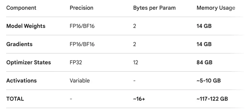
Training LLMs is very costly, both wrt to time and resources.
Challenge
When we fine-tune an LLM, we do not just store the model’s weights.
We also have to store optimizer states, gradients, and activations.
7B parameters LLM
Solution
Instead of retraining the entire \(d_{model} \times d_{model}\) weight matrices,
PEFT methods only update a tiny fraction (often \(<1\%\)) of the parameters while keeping the original “knowledge” of the
pre-trained Transformer frozen.
Key PEFT methods include LoRA (most popular), QLoRA, Prefix Tuning, and Adapter layers.
Low-Rank Adaptation (LoRA)
It freezes the original model weights and injects two small, trainable low-rank matrices into the attention layers.
Reduces trainable parameters by up to 99% while maintaining near-identical performance to full fine-tuning.
Prevents “catastrophic forgetting”.
Attention layers are the primary target for LoRA because they act as the “brain” for context and relationships in Transformers.
By modifying the Attention Mechanism, we change how the model decides which parts of the input are relevant to each other.
While weights of Feed Forward Neural Network and Layer Normalization are frozen to avoid catastrophic forgetting.
Low Rank Matrices
When we train a model, we are looking for a change in weights, which we call \(\Delta W\).
Note: ‘\(r\)’ is the rank, a small integer (e.g., 4, 8, or 16).
PEFT (LoRA) Working
- Initialization:
- Matrix ‘\(B\)’ is initialized to 0.
- Matrix ‘\(A\)’ is initialized with random Gaussian noise.
- At the very start of training,\(BA = 0\), meaning the model starts with the exact same behavior as the original pre-trained model.
- Forward Pass:
- Input ‘\(x\)’ is passed through both the frozen weights and the trainable “adapters” in parallel.
- \(h = Wx + BAx\)
- Back Propagation:
- Gradients are only calculated and updated for matrices ‘\(A\)’ and ‘\(B\)’.
- Because ‘\(r\)’ is so small, we are often training less than 1% of the total parameters.
- Inference:
- After training, we can mathematically “merge” the weights:\(W_{updated} = W + BA\).
- This results in a single matrix of the original size, meaning the model runs just as fast as the original with zero overhead.
Example
\(W_q = d \times d\) and \(B = d \times r\), \(A = r \times d\)
Let, d = 1000, and r = 4.
- Full Matrix (\(W\)): \(1000 \times 1000 = 1,000,000\) parameters
- Matrix B: \(1000 \times 4 = 4,000\) parameters
- Matrix A: \(4 \times 1000 = 4,000\) parameters
- \(\frac{\text{LoRA Parameters}}{\text{Full Parameters}} = \frac{8,000}{1,000,000} = 0.008\)
Therefore, we train only 0.8% of the parameters for that layer.
Across the whole model, this usually results in training ~0.1% to 1%.
12 - BERT
Limitations of Word Vectors
Before 2018, models like Word2Vec and GloVe provided “context-free” embeddings.
The word “bank” had the same vector whether it was a “river bank” or a “bank account”.
Google AI Language team developed, Transformer (encoder only) based language model designed to understand the meaning of words in a text by using the context from both directions.
BERT Architecture (Encoder Only)
BERT Input Representation
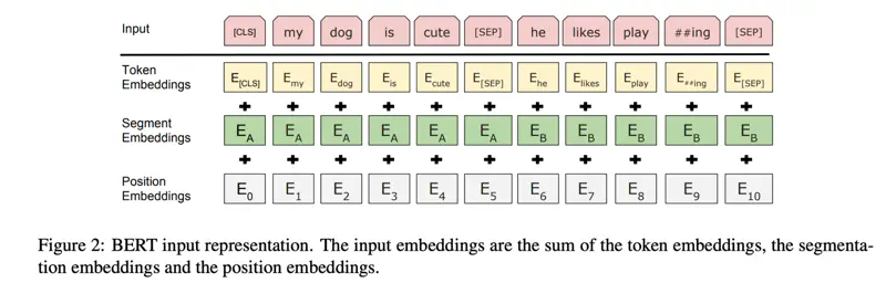
Note: BERT uses WordPiece embeddings (Wu et al., 2016) with a 30,000 token vocabulary.
Research Paper: BERT: Pre-training of Deep Bidirectional Transformers for Language Understanding, Devlin et al., 2018; https://arxiv.org/pdf/1810.04805
Pre-Training
Model is trained on a massive, unlabeled dataset (e.g., internet scale) to learn
general language features, grammar, syntax, and reasoning patterns, using self-supervised learning techniques.
The self-supervised technique used in BERT is ‘Masked Language Modeling’.
Masked Language Modeling
A percentage of tokens in a sentence (typically 15%) are randomly hidden or “masked,”
and the model must predict these missing words using context from both directions (bidirectional).
- Replace the word with [MASK] 80% of the time.
- Replace the word with random word 10 % of the time.
- Keep the same word 10% of the time.
Example

Many important tasks such as Question Answering (QA) and Natural Language Inference (NLI) are based on understanding the relationship between two sentences, which is not directly captured by language modeling.
Pre-train for next sentence prediction task.
- IsNext: 50% of the time B is the actual next sentence that follows A.
- NotNext: 50% of the time it is a random sentence from the corpus.
- [CLS] Classification
- The special token added to the start of every input.
- It acts as a summary representation of the entire sentence, aggregating information via self-attention mechanisms across transformer layers.
- Final hidden state of the [CLS] token (768 dimensions) is passed through a classifier(simple linear layer) to determine if a sentence is positive or negative.
- [SEP] Separator
- Special separator token used to mark the end of a sentence or to explicitly separate two different text segments within a single input sequence.
- e.g. [CLS] Sentence A [SEP] Sentence B [SEP]
- ✅ Search Relevance and Ranking (Google Search): BERT helps Google Search understand the intent and context behind complex, conversational search queries rather than just matching keywords.
- ✅ Question Answering Systems: BERT excels at analyzing large documents to find specific answers, used extensively in chatbots and virtual assistants for customer support.
- ✅ Sentiment Analysis: BERT excels at analyzing social media, product reviews, or customer service logs to determine sentiment, separating positive and negative sentiment in contexts.
- ✅ Named Entity Recognition(NER): It improves the identification of proper nouns, i.e., names, organizations, and locations in unstructured text.
To compare 2 sentences BERT requires both the sentences to be fed to the model.
💡 Finding the most similar pair in a collection of 10,000 sentences requires about 50 million inference computations (~65 hours) with BERT.
❌ The construction of BERT makes it unsuitable for semantic similarity search, such as RAG applications.
Modification of the pre-trained BERT network that use Siamese and triplet network structures to derive semantically meaningful sentence embeddings that can be compared using cosine-similarity.
✅ This reduces the effort for finding the most similar pair from 65 hours with BERT / RoBERTa to about 5 seconds with SBERT, while maintaining the accuracy from BERT.
SBERT Architecture
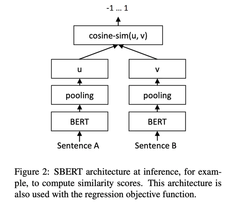
SBERT Pooling
SBERT adds a pooling operation to the output of BERT / RoBERTa to derive a fixed sized (768) sentence embedding.
3 pooling strategies:
- Computing the mean of all output vectors (MEAN-strategy); Default
- Computing a max-over-time of the output vectors (MAX-strategy)
- Using the output of the CLS-token
Research Paper: Sentence-BERT: Sentence Embeddings using Siamese BERT-Networks, Reimers & Gurevych, 2019; https://arxiv.org/pdf/1908.10084