Batch Normalization
3 minute read
Problem
In deep neural networks, during training, as weights update the distribution of input values to hidden layers changes
continuously, also called, ‘internal covariate shift’ (ICS).
This change forces layers to constantly adapt to new input distributions, which :
- slows down training,
- hinders convergence, and
- makes hyper-parameter tuning difficult
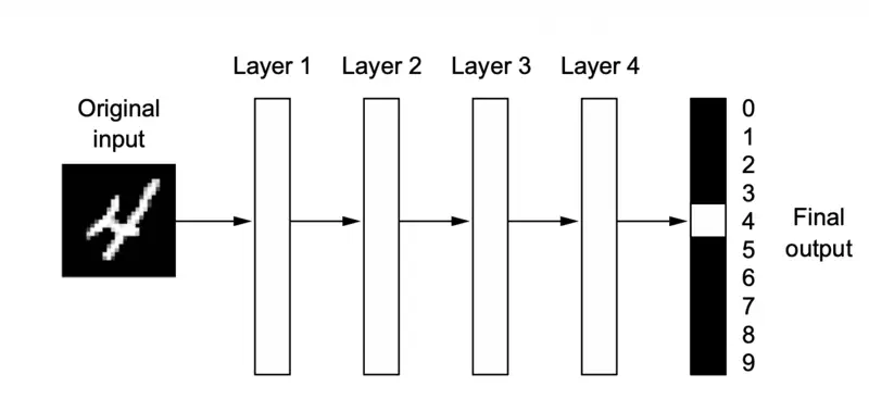
A deep neural network for digit classification
Batch Normalization is a technique to control the variation in the features, such that, they do not vary too much and are bounded (by normalizing the inputs to each layer).
\[ \hat{x}_i = \frac{x_i - \mu_{\mathcal{B}}}{\sqrt{\sigma_{\mathcal{B}}^2 + \epsilon}} \]where, \(\epsilon \approx 10^{-5}\) is a tiny constant to prevent division by zero.
If we always normalize to mean \(\mu\)=0 and variance \(\sigma^2\)=1, we might restrict the layer too much (e.g., forcing everything into the linear region of a Sigmoid function) and the network might lose representational power.
💡 So BatchNorm introduces learnable parameters:
\[y_i = \gamma \hat{x}_i + \beta\]- \(\gamma\) = scaling parameter
- \(\beta\)= shifting parameter
Note: The network can now decide for itself if it wants the mean(\(\mu\)) to be 0 and variance(\(\sigma^2\)) to be 1.
If the optimal state for the network is something else, it can learn the values for ‘\(\gamma\)’ and ‘\(\beta\)’ to undo the normalization.
Inference Time
- During training, mean(\(\mu\)) and variance(\(\sigma^2\)) come from current mini-batch.
- At inference (test) time, we use frozen running averages of the mean(\(\mu\)) and variance(\(\sigma^2\)) calculated during training.
Research Paper: Batch Normalization: Accelerating Deep Network Training by Reducing Internal Covariate Shift, Ioffe & Szegedy, 2015, https://arxiv.org/pdf/1502.03167
- Mitigates changing distributions (internal covariate shift).
- Prevents vanishing/exploding gradients.
- Allows for higher learning rates.
- Smoothing the optimization landscape.
- Acts as a regularizer to reduce overfitting.
- Because BN calculates the mean(\(\mu\)) and variance(\(\sigma^2\)) for each mini-batch, these statistics vary slightly across different batches. This randomness introduces a small amount of noise into the activations, which acts as a regularizer, similar to dropout.
import tensorflow as tf
from tensorflow.keras import layers, models, regularizers
import numpy as np

# 1. Setup Synthetic Data (Binary Classification)
# 1000 samples, 20 features per sample
X = np.random.rand(1000, 20).astype(np.float32)
y = np.random.randint(2, size=(1000, 1)).astype(np.float32)

# 2. Define the Sequential Model
model = models.Sequential([
    # Input Layer
    layers.Input(shape=(20,)),

    # Hidden Layer 1: Dense + L2 Regularization
    layers.Dense(64, kernel_regularizer=regularizers.l2(0.01), name="dense_1"),
    layers.BatchNormalization(name="batch_norm_1"), # Normalizes activations
    layers.Activation('relu'),
    layers.Dropout(0.3, name="dropout_1"),          # Prevents overfitting

    # Hidden Layer 2
    layers.Dense(32, kernel_regularizer=regularizers.l2(0.01), name="dense_2"),
    layers.BatchNormalization(name="batch_norm_2"),
    layers.Activation('relu'),
    layers.Dropout(0.2, name="dropout_2"),

    # Output Layer (Sigmoid for binary probability)
    layers.Dense(1, activation='sigmoid', name="output_layer")
])

# 3. Compile the Model
model.compile(
    optimizer=tf.keras.optimizers.Adam(learning_rate=0.001),
    loss='binary_crossentropy',
    metrics=['accuracy']
)

# 4. Print Architecture & Parameters
print("--- Model Architecture ---")
model.summary()
Output
--- Model Architecture ---
Model: "sequential_23"
┏━━━━━━━━━━━━━━━━━━━━━━━━━━━━━━━━━┳━━━━━━━━━━━━━━━━━━━━━━━━┳━━━━━━━━━━━━━━━┓
┃ Layer (type)                    ┃ Output Shape           ┃       Param # ┃
┡━━━━━━━━━━━━━━━━━━━━━━━━━━━━━━━━━╇━━━━━━━━━━━━━━━━━━━━━━━━╇━━━━━━━━━━━━━━━┩
│ dense_1 (Dense)                 │ (None, 64)             │         1,344 │
├─────────────────────────────────┼────────────────────────┼───────────────┤
│ batch_norm_1                    │ (None, 64)             │           256 │
│ (BatchNormalization)            │                        │               │
├─────────────────────────────────┼────────────────────────┼───────────────┤
│ activation_2 (Activation)       │ (None, 64)             │             0 │
├─────────────────────────────────┼────────────────────────┼───────────────┤
│ dropout_1 (Dropout)             │ (None, 64)             │             0 │
├─────────────────────────────────┼────────────────────────┼───────────────┤
│ dense_2 (Dense)                 │ (None, 32)             │         2,080 │
├─────────────────────────────────┼────────────────────────┼───────────────┤
│ batch_norm_2                    │ (None, 32)             │           128 │
│ (BatchNormalization)            │                        │               │
├─────────────────────────────────┼────────────────────────┼───────────────┤
│ activation_3 (Activation)       │ (None, 32)             │             0 │
├─────────────────────────────────┼────────────────────────┼───────────────┤
│ dropout_2 (Dropout)             │ (None, 32)             │             0 │
├─────────────────────────────────┼────────────────────────┼───────────────┤
│ output_layer (Dense)            │ (None, 1)              │            33 │
└─────────────────────────────────┴────────────────────────┴───────────────┘
 Total params: 3,841 (15.00 KB)
 Trainable params: 3,649 (14.25 KB)
 Non-trainable params: 192 (768.00 B)