Optimization Methods
9 minute read
The loss function surface in deep learning is non-convex, i.e, it has multiple local minima, saddle points,
and plateaus rather than a single, global minimum.
So, in the context of neural network training, we usually do not care about finding the exact (global) minimum of a function,
but seek only to reduce its value sufficiently to obtain good generalization error.
🖼️ Non-Convex Loss Surface Examples
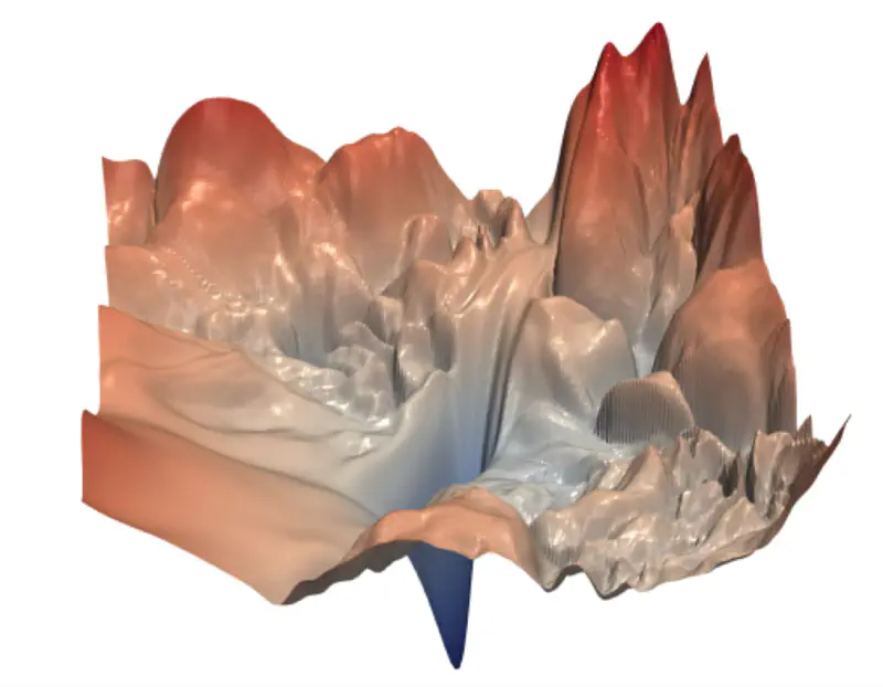
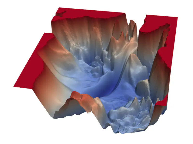
Because of the non-convex loss surface, convergence to a good minimum is often slow, because of multiple reasons:
- Multiple local minima; may not land in a good enough local minima.
- Saddle points; near a saddle point, optimizer barely moves.
- Presence of flat regions (plateaus), where the gradient is near zero, offering minimal guidance for the optimizer.
- “Ravine-like” structure (steep on one side, flat on the other), stochastic gradient descent oscillates uncontrollably.
- Different parameters require different learning rates; e.g, sparse parameters will get very few updates.
Training deep neural networks is inherently complex because of the multiple layers and the vast number of parameters to be updated during training.
Therefore, we need to find ways to accelerate the optimization process.
The optimization process can be accelerated considerably by using stochastic gradient descent (instead of simple gradient descent), i.e, follow the gradient of randomly selected mini-batches downhill.
\[w_{new} = w_{old} - \eta.\text{(average gradient of randomly chosen ‘m' data points)}\]where, \(\eta\) = learning rate
In practice, it is common to decay the learning rate linearly until some pre-defined fixed number of iterations ‘\(\tau\)’.
The primary reason for this approach is to start with a high learning rate to rapidly traverse the loss landscape and escape poor local minima, while later using a small learning rate to fine-tune the parameters and settle into a deeper, more stable minimum without oscillating around it.
\[\eta_k = (1-\alpha)\eta_0 + \alpha\eta_{\tau}\]where, \(\alpha = \frac{k}{\tau}\)
After,’\(\tau\)’ iterations, leave the learning rate \(\eta\) constant.
e.g., \(\eta_0 = 0.1,~ \eta_{\tau}=0.01, \text{ and } \tau=100\)
Say, we have ’n’ samples, and we divide them into mini-batches, such that, each mini-batch has ‘m’<’n’ samples.
- 1 iteration = weight update after computing the gradient of 1 mini-batch
- 1 epoch = one complete pass through the entire training dataset = n/m iterations
- L epochs = L x (n/m) iterations
Note:
- Size ‘m’ of a mini-batch is decided based on the computing resources, such as RAM, GPU, TPU etc., e.g, Nvidia H100 GPU has 80GB RAM.
- In practice, the mini-batch size is chosen to be the largest possible power of 2 that fits within the available GPU memory while still allowing for good model performance.
- Samples in the mini-batches are randomized in every epoch.
Methods to accelerate the optimization process in deep learning:
- Momentum Based; Polyak (1964) | Refined for Deep Learning: Sutskever et al. (2013)
- AdaGrad (Adaptive Gradient); Duchi, Hazan, and Singer (2011)
- RMSProp (Root Mean Square Propagation); Geoffrey Hinton (2012)
- Adam (Adaptive Moment Estimation); Kingma and Ba (2014)
💡 Momentum introduces velocity.
(term borrowed from Physics, where momentum = mass x velocity)
‘Accumulates’ velocity in directions of consistent gradients and cancels out directions that fluctuate.
Algorithm
- For each iteration (t):
- Instead of moving purely by gradient: \[w_{t+1} = w_{t} - \eta . g_t\]
- Accumulate previous gradients, i.e, the velocity (speed + direction): \[ v_{t} = \gamma . v_{t-1} + \eta. g_t\]
- where, \( \gamma \) = momentum coefficient (typically 0.9)
- Update parameter: \[ w_{t+1} = w_{t} - v_{t} \]
Size of the step depends on how large and how aligned are a sequence of gradients.
\[ \begin{aligned} \text{Let, } v_0 &= 0 \\ v_1 &= \gamma. v_0 + \eta.g_0 = \eta.g_0\\ v_2 &= \gamma. v_1 + \eta.g_1 = \gamma (\eta.g_0) + \eta.g_1 \\ v_3 &= \gamma. v_2 + \eta.g_2 = \gamma (\gamma (\eta.g_0) + \eta.g_1 ) + \eta.g_2 = \eta(\gamma^2 g_0 + \gamma g_1 + g_2)\\ v_{k} &= \eta(\gamma^{k-1} g_0 + \gamma^{k-2} g_1 + \dots g_{k-1})\\ \end{aligned} \]If many successive gradients point in exactly the same direction, then we want to take larger steps.
\[ \lim_{k\rightarrow \infty} v_k = \eta.g(1+\gamma+ \gamma^2 + \dots \infty) \]The term inside the bracket, is a geometric progression with the common ratio \(\gamma < 1\).
So, if the momentum algorithm always observes gradient ‘g’, then it will accelerate in the direction of ‘g’, until reaching a terminal velocity where the size of each step is:
\[ \frac{\eta. \lVert g \rVert}{1-\gamma} \]where, \(0 < \gamma < 1\)
Say, if \(\gamma\)= 0.9, then it means to multiply the maximum velocity by 10 relative to a gradient descent algorithm.
🖼️ Momentum Based Optimizer Vs SGD
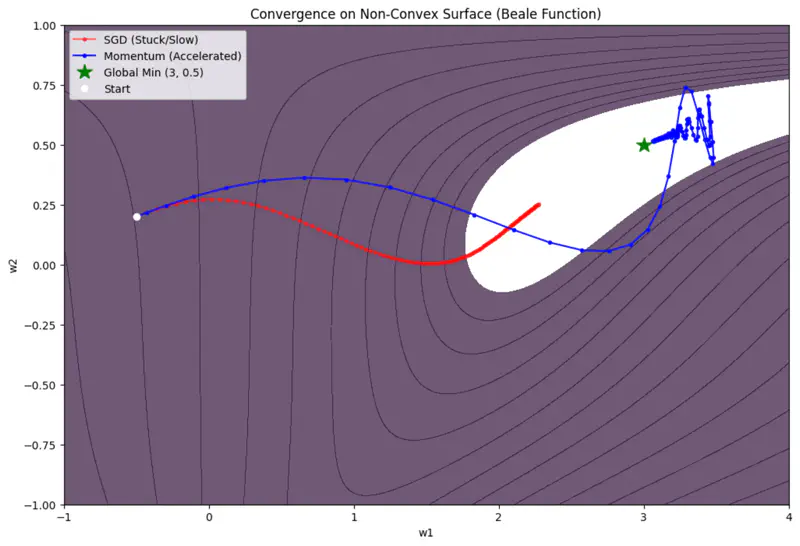
Limitations
- Momentum can be like a heavy ball rolling down a hill; it gathers so much speed that it may overshoot the minima.
- It does not adjust the learning rate based on the importance of specific features.
💡 Scales the learning rate for each parameter based on the historical sum of squares of its gradients.
Problem
In many datasets, some features are frequent while others are sparse.
e.g., Predicting house prices based on certain rare feature, such as, presence of shopping mall.
For most of the houses the value of that feature is 0.
A single learning rate ‘\(\eta\)’ for all parameters is inefficient.
We want larger updates for sparse features and smaller updates for frequent ones.
Algorithm
- For each iteration (t):
- Calculate gradient \(g_t\).
- Accumulate gradients: \[ r_{t} = r_{t-1} + g_t \odot g_t\]
- Update parameter: \[ w_{t+1} = w_{t} - \frac{\eta}{\sqrt{r_t} + \delta} \odot g_t \]
- where, \(\delta\) is small smoothing term (e.g. \(10^{-8}\)) to avoid division by 0.
- if, \(g = \begin{bmatrix} g_1 \\ g_2 \\ \vdots \\ g_d \end{bmatrix} \), then \( g \odot g = \begin{bmatrix} g_1^2 \\ g_2^2 \\ \vdots \\ g_d^2 \end{bmatrix} \) (element wise dot product)
Since, \(r_{t+1} = r_{t} + g_t \odot g_t\), so, for sparse features, we hardly get any gradient updates, so ‘g’ is mostly 0.
Therefore, accumulations ‘r’ is very small.
Since, \(w_{t+1} = w_{t} - \frac{\eta}{\sqrt{r_t} + \delta} \odot g_t\), this implies that, the learning rate is inversely proportional to accumulations ‘r’.
Therefore, sparse features get larger updates, whereas, for weights that are frequent will have very large accumulations,
as a result, the learning rate will start decaying.
Limitation
Vanishing Learning Rate Problem:
Since accumulation of gradients increases monotonically.
This causes the effective learning rate to shrink until it becomes infinitesimally small, effectively ‘killing’
the learning process before the model converges.
💡 Instead of summing all past squared gradients, as in AdaGrad, RMSProp uses an exponentially decaying average to discard history from the extreme past so that it can converge rapidly.
Algorithm
- For each iteration (t):
- Calculate gradient \(g_t\).
- Accumulate gradients: \[ r_{t} = \rho r_{t-1} + (1 - \rho)g_t \odot g_t \]
- Update parameter: \[ w_{t+1} = w_{t} - \frac{\eta}{\sqrt{r_t} + \delta} \odot g_t \]
- where, \(\delta\) is small smoothing term (e.g. \(10^{-8}\)) to avoid division by 0.
- if, \(g = \begin{bmatrix} g_1 \\ g_2 \\ \vdots \\ g_d \end{bmatrix} \), then \( g \odot g = \begin{bmatrix} g_1^2 \\ g_2^2 \\ \vdots \\ g_d^2 \end{bmatrix} \) (element wise dot product)
Since, \(r_{t} = \rho r_{t-1} + (1 - \rho)g_t \odot g_t\), say, if \(\rho = 0.9\), then we trust the historical average 90% and the new gradient only 10%, i.e, \(r_t = 0.9r_{t-1} + 0.1g_t \odot g_t\). \[ r_t = (1-\rho)g_t^2 + \rho(1-\rho)g_{t-1}^2 + \rho^2(1-\rho)g_{t-2}^2 + \dots\]
So, if the algorithm always observes gradient ‘g’, then \(r_t\) becomes:
\[ r_t = (1-\rho)g^2 (1 + \rho + \rho^2 + \dots)\]The term inside the second bracket, is a geometric progression with the common ratio \(\rho < 1\).
Note: \(\rho \) is the decay rate (commonly 0.9 or 0.99).
So, the accumulation of gradient does not grow uncontrollably, as in AdaGrad.
Therefore, the “Vanishing Learning Rate” problem is solved.
Limitation
Lacks the ‘momentum’ component to accelerate through flat regions or dampen oscillations.
💡Adam optimizer combines:
- Adaptive learning rates of RMSProp
- Accelerated convergence of Momentum
Adam calculates an exponential moving average of the gradient (first moment) and the squared gradient (second moment).
It also includes a bias-correction term to account for the fact that these averages are initialized at zero.
Algorithm
- For each iteration (t):
- Calculate gradient \(g_t\).
- Update biased first moment estimate: \[ m_t = \beta_1 m_{t-1} + (1 - \beta_1)g_t \]
- Update biased second raw moment estimate: \[ v_t = \beta_2 v_{t-1} + (1 - \beta_2)g_t^2 \]
- Compute bias-corrected first moment estimate: \[ \hat{m}_t = \frac{m_t}{1 - \beta_1^t} \]
- Compute bias-corrected second raw moment estimate: \[ \hat{v}_t = \frac{v_t}{1 - \beta_2^t} \]
- Update parameter: \[w_{t+1} = w_t - \frac{\eta}{\sqrt{\hat{v}_t} + \epsilon} \hat{m}_t\]
Since, \(m_t = \beta_1 m_{t-1} + (1 - \beta_1)g_t\), say if, \(\beta_1 = 0.9\), then we trust the historical average 90% and the new gradient only 10%, i.e, \(m_t = 0.9m_{t-1} + 0.1g_t\)
Expanding the equation:
\[ m_t = 0.1g_t + 0.9(0.9 m_{t-2} + 0.1 g_{t-1}) = 0.1g_t + 0.09 g_{t-1} + 0.081 g_{t-2} + \dots \]Because the weight drops by a factor of \(\beta_1\) for every step back, the influence of older gradients decays exponentially.
Bias Correction
Bias correction compensates for the fact that the initial estimates of the first and second moments are biased towards zero.
Since \(m_0\) is initialized to zero, \(m_t\) will be close to zero during the initial time steps, especially when \(\beta_1\) is close to 1.
Common defaults: \(\beta_1 = 0.9 ,~ \beta_2 = 0.999,~ \eta = 0.001\)
Advantages
✅ Faster convergence.
✅ Require little to no adjustment of its default hyper-parameter values.
✅ It is computationally efficient, requires little memory to store moving averages.
✅ Adam is currently the ‘default’ optimizer for most deep learning tasks.