XOR Problem
5 minute read
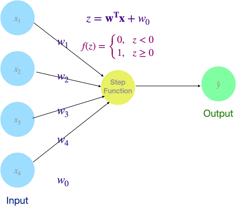
Simplest form of an artificial neural network, acting as a single-layer binary classifier that categorizes input data into one of two groups.
It serves as a mathematical model of a biological neuron, receiving multiple signals (inputs), weighting their importance, and deciding whether to ‘fire’ (output 1) or stay ‘inactive’ (output 0).
🖼️ Perceptron
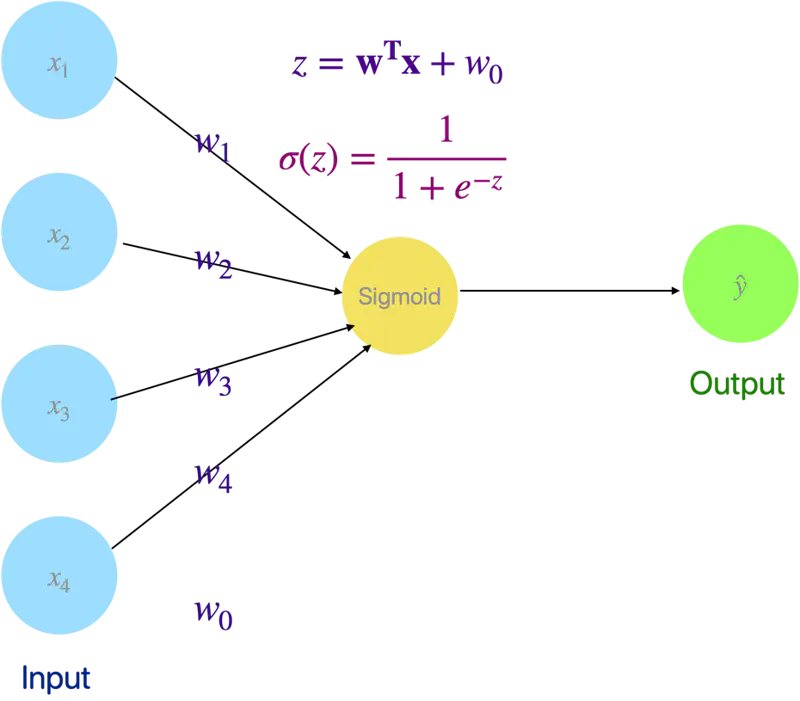
💡 Even Logistic Regression is a simple neural network with a sigmoid activation (instead of step function as in Perceptron).
🖼️ Logistic Regression as a Neural Network
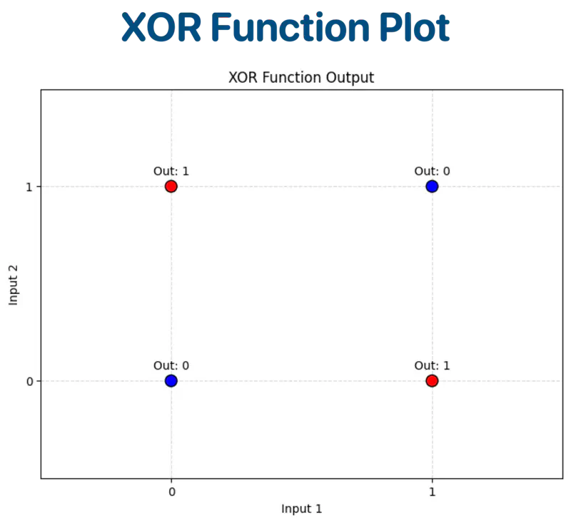
XOR Function:
| Input A | Input B | Output (A ⊕ B) |
|---|---|---|
| 0 | 0 | 0 |
| 0 | 1 | 1 |
| 1 | 0 | 1 |
| 1 | 1 | 0 |
Let’s plot the input and output on a graph for visualization.
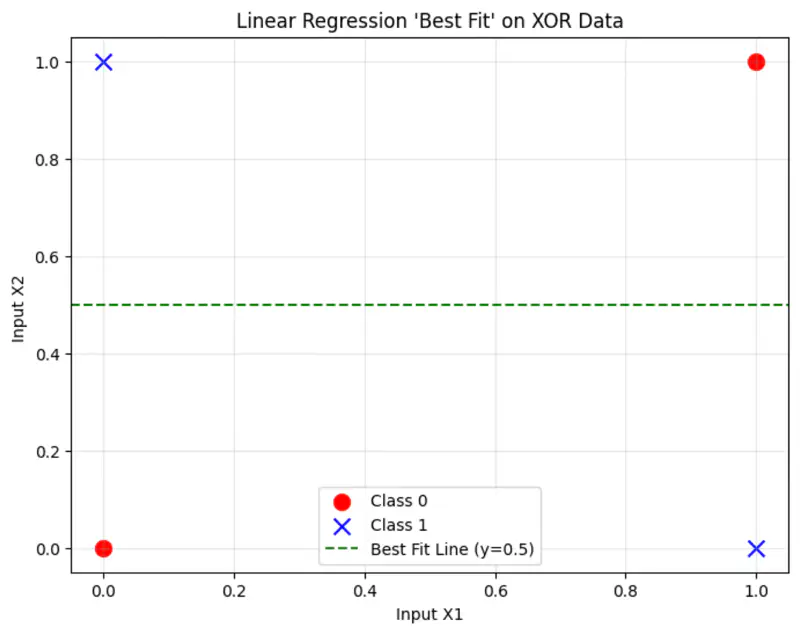
Linear Regression
The cost function:
where, \(\hat{y_i} = \mathbf{w^Tx} + w_0\)
Solving the normal equations, we get:
\(\mathbf{w = 0} , w_0 = 0.5\)
This implies, whatever is the input, we always get 0.5 as output,
because linear regression is trying to fit the best line to the data, which in this case will be mid-way between the points.
And, that definitely is not the correct solution.
Logistic Regression
Similarly logistic regression can not find a single linear decision boundary to separate the 4 XOR outputs.
❌ No straight line can separate the XOR points.
Therefore, a linear model is not sufficient to represent the XOR function.
So, we need more than 1 neuron to solve the XOR problem (because logistic regression is a neural network with a single neuron).
Let’s solve the XOR problem with a simple neural network with 2 neurons (1 hidden layer) and ReLU activation function.
1 Hidden layer and 2 Neurons
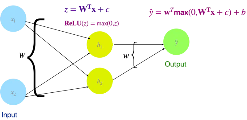
We will use linear algebra to demonstrate one of solutions to the problem.
Let input = X and output = Y.
Out of many possible solutions, let’s look at the below solution:
Weight and bias of hidden layer:
Output of hidden layer:
\[z = XW + c\]\[ XW = \begin{bmatrix} 0 & 0 \\ 0 & 1 \\ 1 & 0 \\ 1 & 1 \end{bmatrix} \begin{bmatrix} 1 & 1 \\ 1 & 1 \end{bmatrix} = \begin{bmatrix} 0 & 0 \\ 1 & 1 \\ 1 & 1 \\ 2 & 2 \end{bmatrix} \]\[ z = \begin{bmatrix} 0 & 0 \\ 1 & 1 \\ 1 & 1 \\ 2 & 2 \end{bmatrix} + \begin{bmatrix} 0 & -1 \\ 0 & -1 \\ 0 & -1 \\ 0 & -1 \end{bmatrix} = \begin{bmatrix} 0 & -1 \\ 1 & 0 \\ 1 & 0 \\ 2 & 1 \end{bmatrix} \]Now, lets apply ReLU activation function to the output ‘z’ of the hidden layer:
\[ReLU(z) = \begin{bmatrix} 0 & 0 \\ 1 & 0 \\ 1 & 0 \\ 2 & 1 \end{bmatrix}\]Applying ReLU non-linearity, changes the position of the points in the hidden space and now the points can be separated by a line.
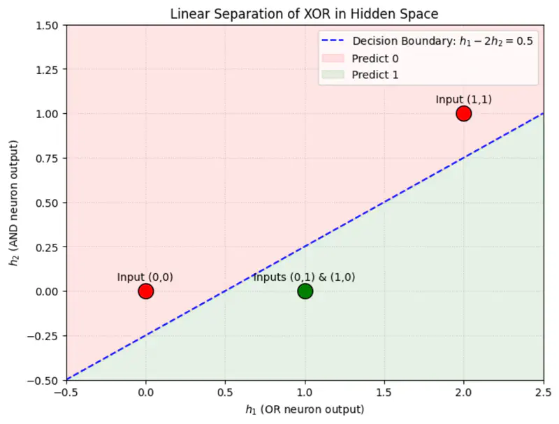
Weight and bias of output layer:
\[\mathbf{w} = \begin{bmatrix} 1 \\ -2 \end{bmatrix}, \quad b = 0\]Output:
\[\hat{y} = \mathbf{w} ~ \text{max}(0, ~ XW + c) + b\]\[\hat{y} = \begin{bmatrix} 0 & 0 \\ 1 & 0 \\ 1 & 0 \\ 2 & 1 \end{bmatrix} \begin{bmatrix} 1 \\ -2 \end{bmatrix} = \begin{bmatrix} 0 \\ 1 \\ 1 \\ 0 \end{bmatrix}\]Therefore, we can see that we have got the expected output for XOR function.
import tensorflow as tf
import numpy as np

# 1. XOR Data
X = np.array([[0, 0], [0, 1], [1, 0], [1, 1]], dtype=np.float32)
y = np.array([[0], [1], [1], [0]], dtype=np.float32)

# 2. Build the Model (2 Hidden Neurons)
model = tf.keras.Sequential([
    tf.keras.layers.Dense(2, activation='leaky_relu',
                         kernel_initializer='he_normal',
                         input_shape=(2,), name='hidden_layer'),
    # Output layer (Linear for MSE)
    tf.keras.layers.Dense(1, name='output_layer')
])

print("--- Model Architecture ---")
model.summary()

# 3. Compile
model.compile(optimizer=tf.keras.optimizers.Adam(learning_rate=0.05), loss='mse')

# 4. Train
print("Training XOR Neural Network ...")
model.fit(X, y, epochs=100, verbose=0)

# 5. Extract and Print Final Weights
weights = model.get_weights()
W, c, w_out, b = weights

print("\n--- Final Weights (W) ---")
print(W)
print(f"\nHidden Bias (c): {c}")
print(f"\nOutput Weights (w): \n{w_out}")
print(f"Output Bias (b): {b}")

# 6. Predictions
print("\n--- Final Predictions ---")
preds = model.predict(X)
for i in range(len(X)):
    print(f"Input: {X[i]} | Raw Output: {preds[i][0]:.4f} | Rounded: {int(np.round(preds[i][0]))}")
Output:
--- Model Architecture ---
Model: "sequential_19"
┏━━━━━━━━━━━━━━━━━━━━━━━━━━━━━━━━━┳━━━━━━━━━━━━━━━━━━━━━━━━┳━━━━━━━━━━━━━━━┓
┃ Layer (type)                    ┃ Output Shape           ┃       Param # ┃
┡━━━━━━━━━━━━━━━━━━━━━━━━━━━━━━━━━╇━━━━━━━━━━━━━━━━━━━━━━━━╇━━━━━━━━━━━━━━━┩
│ hidden_layer (Dense)            │ (None, 2)              │             6 │
├─────────────────────────────────┼────────────────────────┼───────────────┤
│ output_layer (Dense)            │ (None, 1)              │             3 │
└─────────────────────────────────┴────────────────────────┴───────────────┘
 Total params: 9 (36.00 B)
 Trainable params: 9 (36.00 B)
 Non-trainable params: 0 (0.00 B)
Training XOR Neural Network ...

--- Final Weights (W) ---
[[-1.1186169  1.8888004]
 [ 1.0687382 -1.8048155]]

Hidden Bias (c): [-0.20543203 -0.18170778]

Output Weights (w):
[[1.3961141]
 [0.7466789]]
Output Bias (b): [0.0938225]

--- Final Predictions ---
1/1 ━━━━━━━━━━━━━━━━━━━━ 0s 105ms/step
Input: [0. 0.] | Raw Output: 0.0093 | Rounded: 0
Input: [0. 1.] | Raw Output: 1.0024 | Rounded: 1
Input: [1. 0.] | Raw Output: 0.9988 | Rounded: 1
Input: [1. 1.] | Raw Output: 0.0079 | Rounded: 0