Regularization
7 minute read
In ‘Deep Learning’ before thinking of regularization we make sure that the model is able to overfit on the training data
and then later take steps to prevent overfitting.
Overfitting on training data ensures that the model training is successful and is not under-fit, i.e:
- No coding error.
- Layers are all connected and have sufficient capacity to learn the complexity in data.
- Initialization parameters of gradient descent are fine, so that convergence to a local minima occurs.
- Model is trained for enough iterations/epochs.
Note: Overfitting on training data => very low training loss.
Once, we have made sure that the deep learning model is overfitting, now we test the model performance against a separate validation dataset, and if the performance on validation set is poor, this implies that:
- Training and Validation data distributions are different, or
- Overfitting on training data.
Data Augmentation
The best way to make a machine learning model generalize better is to train it on more data.
Of course, in practice, the amount of data we have is limited.
One way to get around this problem is to create fake data from the existing data and add it to the training set.Regularization
- L2 Regularization (Weight Decay)
- Early Stopping
- Dropout
Adds a penalty term proportional to the square of the magnitude of weights to the loss function.
- It prevents overfitting by forcing weight values to be small, encouraging a smoother, simpler model that generalizes better to new data.
- Weights ‘decay’ toward zero at every step, which is why it’s often called ‘Weight Decay’. \[ \underset{w}{\mathrm{min}}\ J_{reg}(w) = \underset{w}{\mathrm{min}}\ J(w) + \lambda.\sum_{j=1}^n \Vert w_j \Vert_2^2 \]
Note: Most modern optimizers (like AdamW) implement this by default to keep weights small and prevent overfitting.
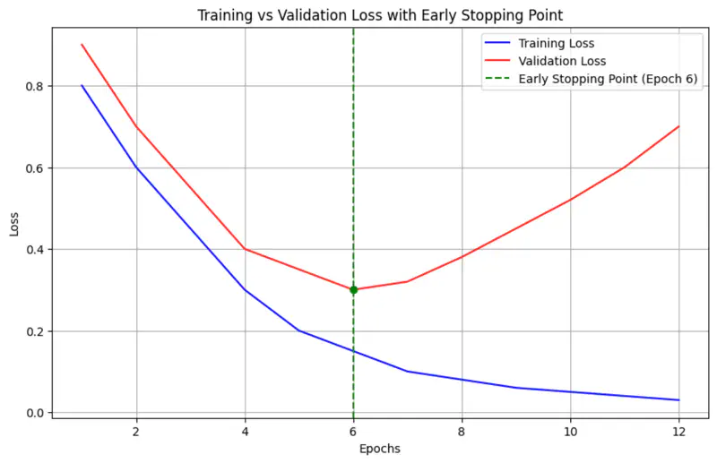
Early stopping is a ‘free’ regularization technique that relies on monitoring the model’s performance on a separate validation set during training.
As training progresses, the error on both training and validation sets usually decreases.
However, at some point, the model begins to ‘memorize’ the training data.
While the training error continues to drop, the validation error starts to rise.
Early stopping halts the training at the precise moment the validation error is at its minimum.
- e.g. if validation loss does not improve for 5 epochs, stop training.
Code
# 1. Define the EarlyStopping callback
# Monitors 'val_loss' and stops if no improvement for 3 epochs.
# restore_best_weights=True ensures you get the model from the best epoch.
early_stop_callback = EarlyStopping(
    monitor='val_loss',
 patience=3,
    restore_best_weights=True
)

# 2. Create a simple model
model = Sequential([
    Dense(10, activation='relu', input_shape=(5,), name="hidden_1", kernel_initializer="he_normal"),
    Dense(1, activation='sigmoid', name="output")
])
model.compile(optimizer='adam', loss='binary_crossentropy', metrics=['accuracy'])


# 3. Train the model with the EarlyStopping callback
# The 'callbacks' argument accepts a list of callbacks.
history = model.fit(
    X_train, y_train,
    epochs=100, # Set a large number of epochs
    validation_data=(X_val, y_val),
 callbacks=[early_stop_callback], # Pass the callback here
    verbose=1
)
Output
Epoch 22/100
4/4 ━━━━━━━━━━━━━━━━━━━━ 0s 23ms/step - accuracy: 0.6100 - loss: 0.6458 - val_accuracy: 0.6000 - val_loss: 0.7082
Epoch 23/100
4/4 ━━━━━━━━━━━━━━━━━━━━ 0s 23ms/step - accuracy: 0.6200 - loss: 0.6450 - val_accuracy: 0.6000 - val_loss: 0.7076
Epoch 24/100
4/4 ━━━━━━━━━━━━━━━━━━━━ 0s 23ms/step - accuracy: 0.6200 - loss: 0.6450 - val_accuracy: 0.6000 - val_loss: 0.7070
Epoch 25/100
4/4 ━━━━━━━━━━━━━━━━━━━━ 0s 23ms/step - accuracy: 0.6200 - loss: 0.6449 - val_accuracy: 0.6000 - val_loss: 0.7079
Epoch 26/100
4/4 ━━━━━━━━━━━━━━━━━━━━ 0s 23ms/step - accuracy: 0.6200 - loss: 0.6446 - val_accuracy: 0.6000 - val_loss: 0.7089
Epoch 27/100
4/4 ━━━━━━━━━━━━━━━━━━━━ 0s 24ms/step - accuracy: 0.6200 - loss: 0.6447 - val_accuracy: 0.6000 - val_loss: 0.7094
Training stopped early after 27 epochs.
Ensemble
Ensemble models reduce overfitting by combining the predictions of multiple diverse models, which reduces the overall
variance of the final model.
Note: If variance of each model is \(\sigma^2 \) then the combined variance of ensemble will be \(\frac{\sigma^2}{k}\).
Read more about Average Variance of Ensemble
Problem
But training multiple different ‘deep learning’ models is costly, also at runtime we need to get the predictions from
all ‘k’ models and take the average of them, which may be time-consuming.
💡 Dropout provides an inexpensive approximation to training and running an ensemble of models.
Randomly remove non-output neurons, i.e, input or hidden layer neurons from the network during every mini-batch (only for that mini-batch) training.
Note: Possible subnetworks = \(2^{n}\), where ’n’ is number of neurons in the input and hidden layers.
Research Paper: Improving neural networks by preventing co-adaptation of feature detectors, Hinton et al., 2012, https://arxiv.org/pdf/1207.0580
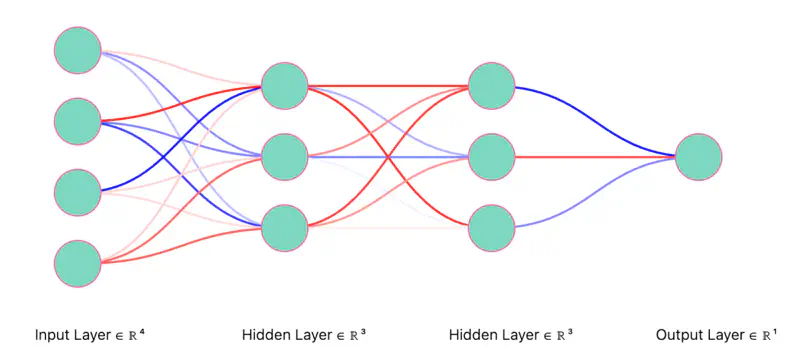
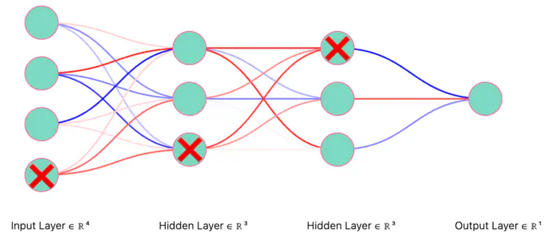
Let’s understand Dropout using the example below.
We will start with a fully connected neural network and randomly dropout(turn-off) neurons.
Fully Connected Neural Network
Dropout Neurons Randomly (iteration 1)
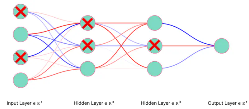
Thinned Network (iteration 1)
Note: Only the “weights” corresponding to retained neurons will be updated in each iteration (mini-batch).
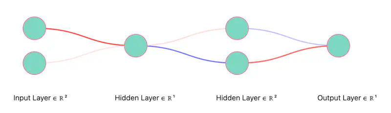
Dropout Neurons Randomly (iteration 2)
Thinned Network (iteration 2)
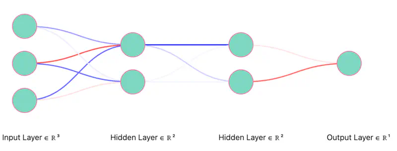
Note: Only the “weights” corresponding to retained neurons will be updated in each iteration (mini-batch).
Since, all neurons are not present in every iteration, so all the weights will not be updated, thus preventing over-fitting.
- We can think of removal of hidden neurons as adding some form of random noise to features.
- Removal of input neurons as input variations.
- All of the above things prevent over-fitting.
Say probability of retaining a neuron,
p(hidden neuron) = 0.6 and p(input neuron) = 0.8
Generate a random number \(r_i \in [0,1]\), if \(r_i \le 0.8\), then retain the input neuron, else drop it; this corresponds to a 80% retention probability.
Co-adaptation in deep learning occurs when neurons become overly dependent on others to correct errors, leading to fragile, overfitted models that perform poorly on new data.
💡 Dropout prevents co-adaptation.
- No single neuron can rely on the presence of another specific neuron to correct its errors.
- This forces every neuron to learn features independently.
Since, each neuron is present in the network with probability ‘p’, so the corresponding outgoing weights of the neuron are scaled by the factor ‘p’ to account for the presence of the that neuron in the network during training.
💡 At inference time we scale the weights.

Note: No clear justification for doing this.
import tensorflow as tf
from tensorflow.keras import layers, regularizers, models
import numpy as np

# Create some dummy data for demonstration purposes
X_train = np.random.rand(1000, 32)
y_train = np.random.rand(1000, 1)
X_val = np.random.rand(200, 32)
y_val = np.random.rand(200, 1)

# Define the L2 regularization strength (e.g., 0.0001)
l2_strength = 1e-4

# Create a Sequential model with L2 regularization and Dropout layers
model = models.Sequential([
    # Add a Dense layer with L2 regularization
    layers.Dense(128, activation='relu',
              kernel_regularizer=regularizers.l2(l2_strength),
                 input_shape=(32,)),

    # Add a Dropout layer with a dropout rate of 30%
 layers.Dropout(0.3),

    # Another Dense layer with L2 regularization
    layers.Dense(64, activation='relu',
                 kernel_regularizer=regularizers.l2(l2_strength)),

    # Another Dropout layer with a dropout rate of 20%
 layers.Dropout(0.2),

    # Output layer
    layers.Dense(1, activation='linear')
])

# Compile the model
model.compile(optimizer='adam',
              loss='mse', # Using Mean Squared Error loss for a regression example
              metrics=['mae']) # Mean Absolute Error as a metric

# Display the model summary
model.summary()

# Train the model (optional, for a complete example)
# history = model.fit(X_train, y_train, epochs=10, validation_data=(X_val, y_val), verbose=1)
Output
------Model Architecture-------
Model: "sequential_21"
┏━━━━━━━━━━━━━━━━━━━━━━━━━━━━━━━━━┳━━━━━━━━━━━━━━━━━━━━━━━━┳━━━━━━━━━━━━━━━┓
┃ Layer (type)                    ┃ Output Shape           ┃       Param # ┃
┡━━━━━━━━━━━━━━━━━━━━━━━━━━━━━━━━━╇━━━━━━━━━━━━━━━━━━━━━━━━╇━━━━━━━━━━━━━━━┩
│ dense_3 (Dense)                 │ (None, 128)            │         4,224 │
├─────────────────────────────────┼────────────────────────┼───────────────┤
│ dropout_2 (Dropout)             │ (None, 128)            │             0 │
├─────────────────────────────────┼────────────────────────┼───────────────┤
│ dense_4 (Dense)                 │ (None, 64)             │         8,256 │
├─────────────────────────────────┼────────────────────────┼───────────────┤
│ dropout_3 (Dropout)             │ (None, 64)             │             0 │
├─────────────────────────────────┼────────────────────────┼───────────────┤
│ dense_5 (Dense)                 │ (None, 1)              │            65 │
└─────────────────────────────────┴────────────────────────┴───────────────┘
 Total params: 12,545 (49.00 KB)
 Trainable params: 12,545 (49.00 KB)
 Non-trainable params: 0 (0.00 B)