GBDT Example
3 minute read
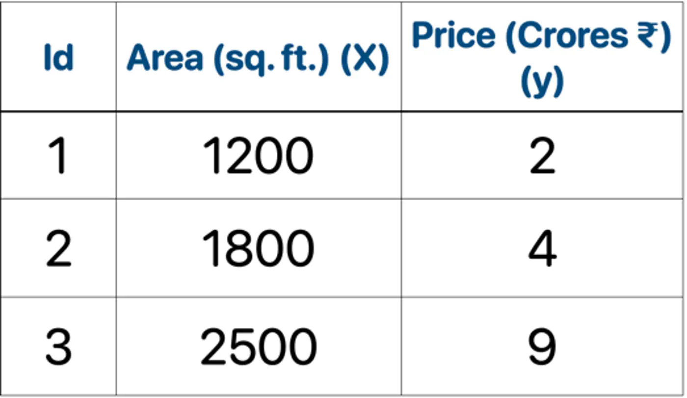
Gradient Boosted Decision Tree (GBDT) is a decision tree based implementation of Gradient Boosting Machine (GBM).
GBM treats the final model \(F_m(x)\) as weighted 🏋️♀️ sum of ‘m’ weak learners (decision trees):
\[ F_{M}(x)=\underbrace{F_{0}(x)}_{\text{Initial\ Guess}}+\nu \sum _{m=1}^{M}\underbrace{\left(\sum _{j=1}^{J_{m}}\gamma _{jm}\mathbb{I}(x\in R_{jm})\right)}_{\text{Decision\ Tree\ }h_{m}(x)}\]- \(F_0(x)\): The initial base model (usually a constant).
- M: The total number of boosting iterations (number of trees).
- \(\gamma_{jm}\)(Leaf Weight): The optimized value for leaf in tree .
- \(\nu\)(Nu): The Learning Rate or Shrinkage; prevent overfitting.
- \(\mathbb{I}(x\in R_{jm})\): ‘Indicator Function’; It is 1 if data point falls into leaf of the tree, and 0 otherwise.
- \(R_{jm}\)(Regions): Region of \(j_{th}\) leaf in \(m_{th}\)tree.
- Step 1: Initialization.
- Step 2: Iterative loop 🔁 : for i=1 to m.
- 2.1: Calculate pseudo residuals ‘\(r_{im}\)'.
- 2.2: Fit a regression tree 🌲‘\(h_m(x)\)'.
- 2.3:Compute leaf 🍃weights 🏋️♀️ ‘\(\gamma_{jm}\)'.
- 2.4:Update the model.
👉Loss = MSE, Learning rate (\(\nu\)) = 0.5
- Initialization : \(F_0(x) = mean(2,4,9) = 5.0\)
- Iteration 1(m=1):
2.1: Calculate residuals ‘\(r_{i1}\)'
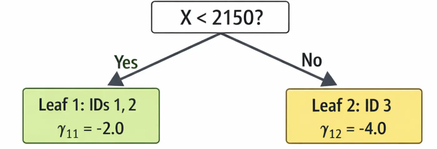
\[\begin{aligned} r_{11} &= 2-5 = -3.0 \\ r_{21} &= 4-5 = -1.0 \\ r_{31} &= 9-5 = 4.0 \\ \end{aligned} \]2.2: Fit tree(\(h_1\)); Split at X<2150 (midpoint of 1800 and 2500)
2.3: Compute leaf weights \(\gamma_{j1}\)
- Y-> Leaf 1: Ids 1, 2 ( \(\gamma_{11}\)= -2.0)
- N-> Leaf 2: Id 3 ( \(\gamma_{21}\)= 4.0)
2.4: Update predictions (\(F_1 = F_0 + 0.5 \cdot \gamma\))
\[ \begin{aligned} F_1(x_1) &= 5.0 + 0.5(-2.0) = \mathbf{4.0}\ \\F_1(x_2) &= 5.0 + 0.5(-2.0) = \mathbf{4.0}\ \\F_1(x_3) &= 5.0 + 0.5(4.0) = \mathbf{7.0}\ \\ \end{aligned} \]Tree 1:
- Iteration 2(m=2):
2.1: Calculate residuals ‘\(r_{i2}\)'
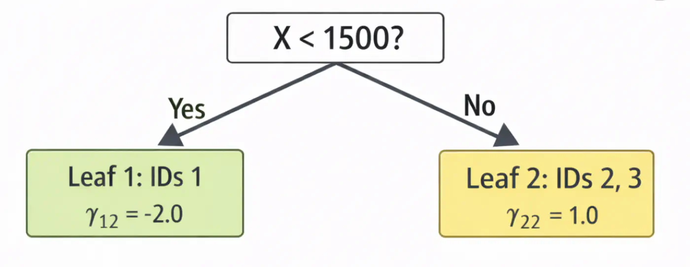
\[ \begin{aligned} r_{12} &= 2-4.0 = -2.0 \\ r_{22} &= 4-4.0 = 0.0 \\ r_{32} &= 9-7.0 = 2.0 \\ \end{aligned} \]2.2: Fit tree(\(h_2\)); Split at X<1500 (midpoint of 1200 and 1800)
2.3: Compute leaf weights \(\gamma_{j2}\)
- Y-> Leaf 1: Ids 1 ( \(\gamma_{12}\)= -2.0)
- N-> Leaf 2: Id 2, 3 ( \(\gamma_{22}\)= 1.0)
2.4: Update predictions (\(F_1 = F_0 + 0.5 \cdot \gamma\))
\[ \begin{aligned} F_2(x_1) &= 4.0 + 0.5(-2.0) = \mathbf{3.0} \\F_2(x_2) &= 4.0 + 0.5(1.0) = \mathbf{4.5} \\ F_2(x_3) &= 7.0 + 0.5(1.0) = \mathbf{7.5}\ \\ \end{aligned} \]Tree 2:
Note: We can keep adding more trees with every iteration;
ideally, learning rate \(\nu\) is small, say 0.1, so that we do not overshoot and converge slowly.
Let’s predict the price of a house with area = 2000 sq. ft.
- \(F_{0}=5.0\)
- Pass though tree 1 (\(h_1\)): is 2000 < 2150 ? Yes, \(\gamma_{11}\)= -2.0
- Contribution (\(h_1\)) = 0.5 x (-2.0) = -1.0
- Pass though tree 2 (\(h_2\)): is 2000 < 1500 ? No, \(\gamma_{22}\) = 1.0
- Contribution(\(h_2\)) = 0.5 x (1.0) = 0.5
- Final prediction = 5.0 - 1.0 + 0.5 = 4.5
Therefore, the price of a house with area = 2000 sq. ft is Rs 4.5 crores, which is very close.
In just 2 iterations, although with higher learning rate (\(\nu=0.5\)), we were able to get a fairly good estimate.
End of Section