Gradient Descent
3 minute read
Minimize the cost function.
\[J(w)=\frac{1}{2n}(y-Xw)^{2}\]Note: The 1/2 term is included simply to make the derivative cleaner (it cancels out the 2 from the square).
Normal Equation (Closed-form solution) jumps straight to the optimal point in one step.
\[w=(X^{T}X)^{-1}X^{T}y\]But it is not always feasible and computationally expensive (due to inverse calculation)
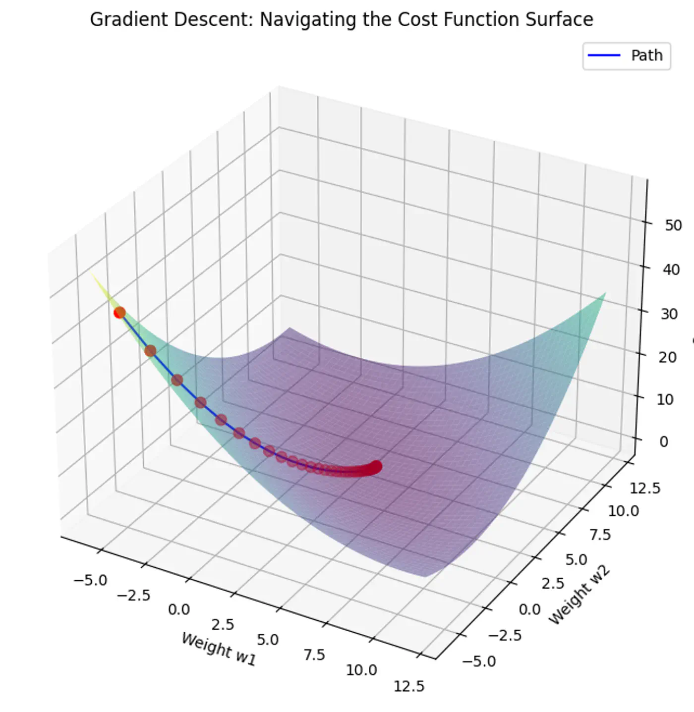
An iterative optimization algorithm slowly nudges parameters ‘w’ towards a value that minimize the costfunction.
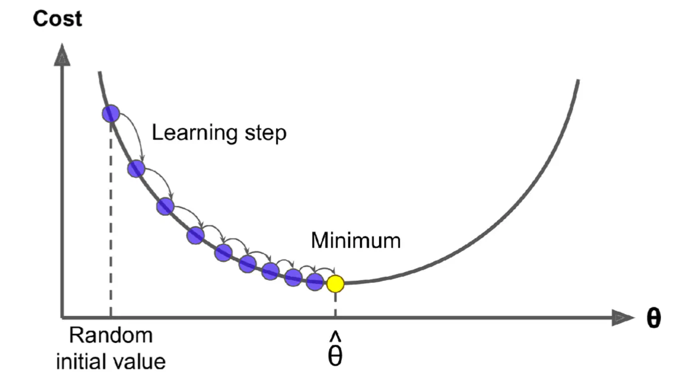
- Initialize the weights/parameters with random values.
- Calculate the gradient of the cost function at current parameter values.
- Update the parameters using the gradient. \[ w_{new} = w_{old} - \eta \frac{\partial{J(w)}}{\partial{w_{old}}} \] \( \eta \) = learning rate or step size to take for each parameter update.
- Repeat steps 2 and 3 iteratively until convergence (to minima).
Applying chain rule:
\[ \begin{align*} &\text{Let } u = (y - Xw) \\ &\text{Derivative of } u^2 \text{ w.r.t 'w' }= 2u.\frac{\partial{u}}{\partial{w}} \\ \frac{\partial{(\frac{1}{2n} (y - Xw)^2)}}{\partial{w}} &= \frac{1}{\cancel2n}.\cancel2(y - Xw).\frac{\partial{(y - Xw)}}{\partial{w}} \\ &= \frac{1}{n}(y - Xw).X^T.(-1) \\ \therefore \frac{\partial{J(w)}}{\partial{w}} &= \frac{1}{n}X^T(Xw - y) \end{align*} \]Note: \(\frac{∂(a^{T}x)}{∂x}=a\)
Update parameter using gradient:
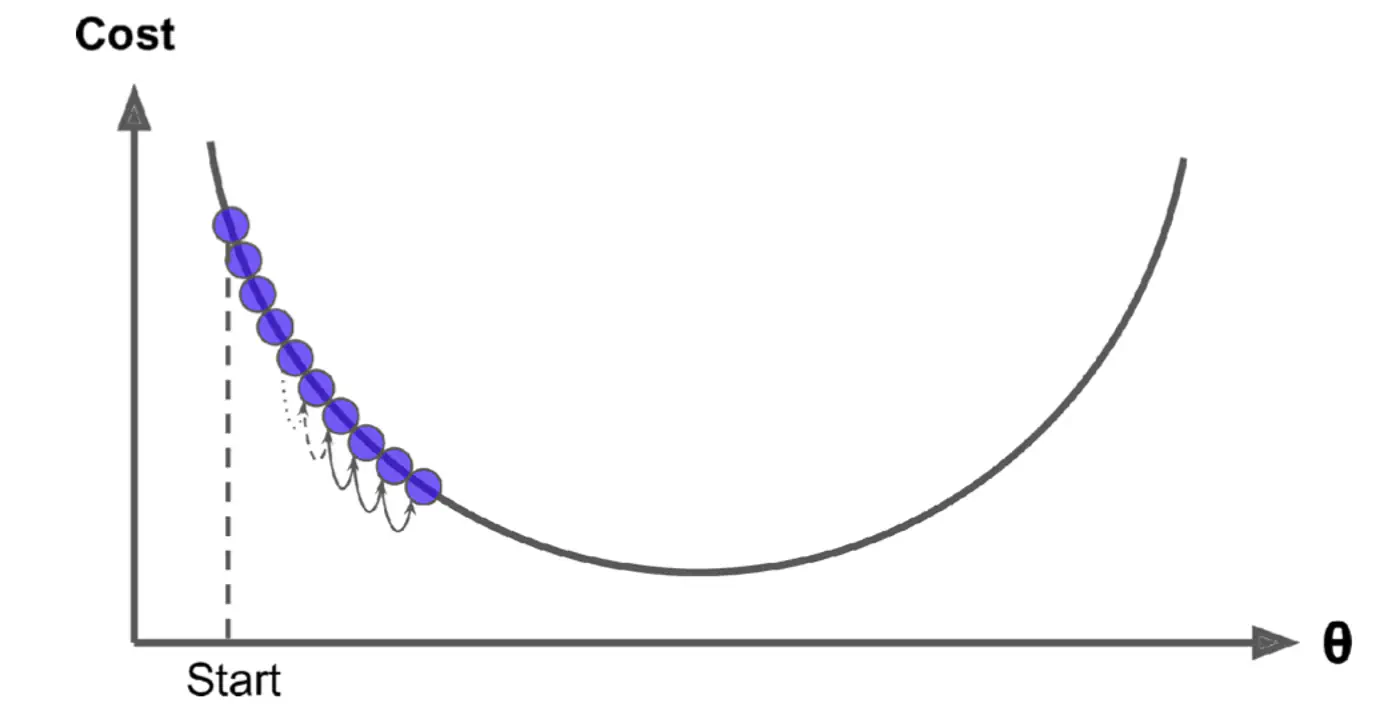
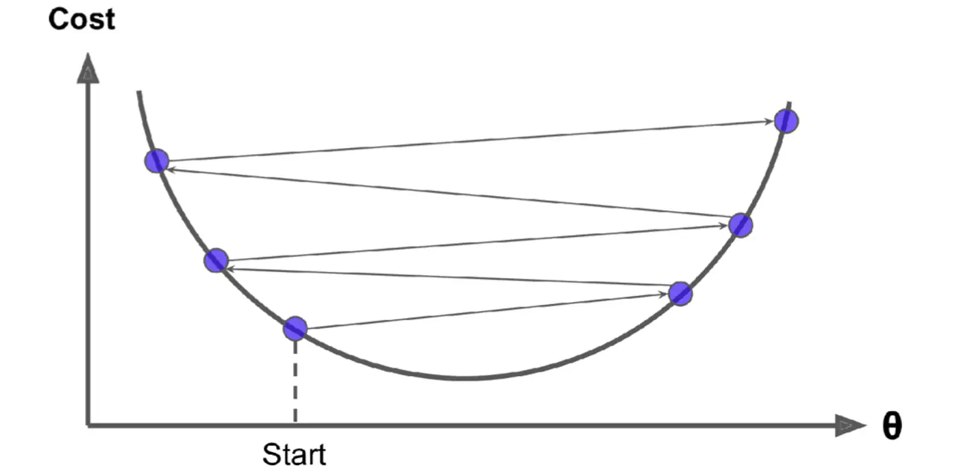
\[ w_{new} = w_{old} - \eta'. X^T(Xw - y) \]- Most important hyper parameter of gradient descent.
- Dictates the size of the steps taken down the cost function surface.
Small \(\eta\) ->
Large \(\eta\) ->
- Learning Rate Schedule:
The learning rate is decayed (reduced) over time.
Large steps initially and fine-tuning near the minimum, e.g., step decay or exponential decay. - Adaptive Learning Rate Methods:
Automatically adjust the learning rate for each parameter ‘w’ based on the history of gradients.
Preferred in modern deep learning as they require less manual tuning, e.g., Adagrad, RMSprop, and Adam.
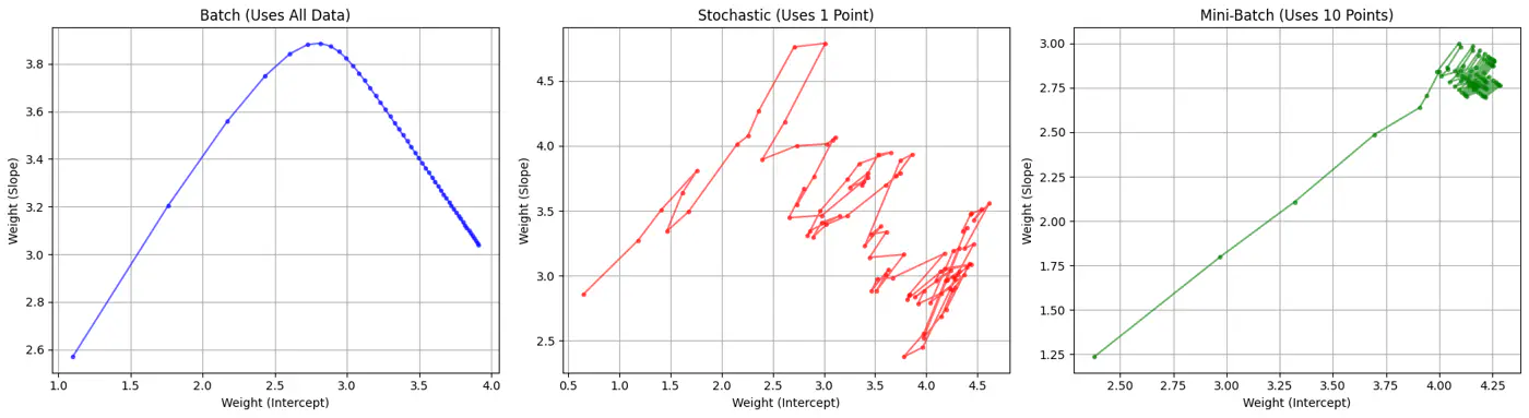
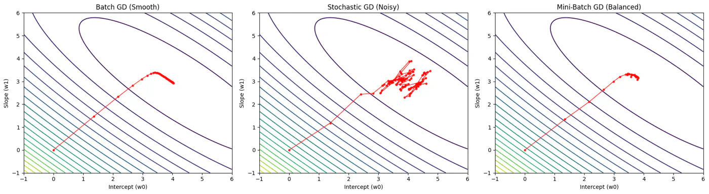
Batch, Stochastic, Mini-Batch are classified by data usage for gradient calculation in each iteration.
- Batch Gradient Descent (BGD): Entire Dataset
- Stochastic Gradient Descent (SGD): Random Point
- Mini-Batch Gradient Descent (MBGD): Subset
Computes the gradient using all the data points in the dataset for parameter update in each iteration.
\[w_{new} = w_{old} - \eta.\text{(average of all ’n’ gradients)}\]Key Points:
- Slow steps towards convergence, i.e, TC = O(n).
- Smooth, direct path towards minima.
- Minimum number of steps/iterations.
- Not suitable for large datasets; impractical for Deep Learning, as n = millions/billions.
Uses only 1 data point selected randomly from dataset to compute gradient for parameter update in each iteration.
\[w_{new} = w_{old} - \eta.\text{(gradient at any random data point)}\]Key Points:
- Computationally fastest per step; TC = O(1).
- Highly noisy, zig-zag path to minima.
- High variance in gradient estimation makes path to minima volatile, requiring a careful decay of learning rate to ensure convergence to minima.
- Uses small randomly selected subsets of dataset, called mini-batch, (1<k<n), to compute gradient for parameter update in each iteration. \[w_{new} = w_{old} - \eta.\text{(average gradient of ‘k' data points)}\]
Key Points:
- Moderate time consumption per step; TC = O(k<n).
- Less noisy, and more reliable convergence than stochastic gradient descent.
- More efficient and faster than batch gradient descent.
- Standard optimization algorithm for Deep Learning.Note: Vectorization on GPUs allows for parallel processing of mini-batches; also GPUs are the reason for the mini-batch size to be a power of 2.