Linear Regression
6 minute read
Let’s understand linear regression using an example to predict salary.
Predict the salary of an IT employee, based on various factors, such as, years of experience, domain, role, etc.
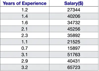
Let’s start with a simple problem and predict the salary using only one input feature.
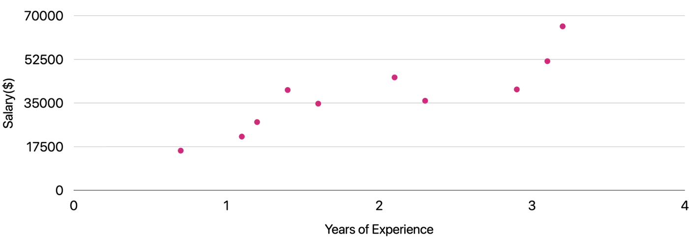
Goal : Find the line of best fit.
Plot: Salary vs Years of Experience
\[y = mx + c = w_1x + w_0\]Slope = \(m = w_1 \)
Intercept = \(c = w_0\)
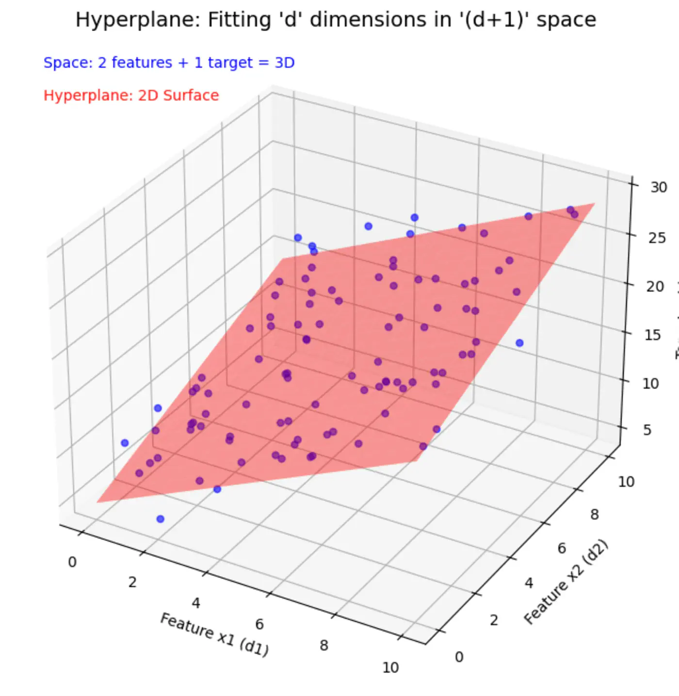
Similarly, if we include other factors/features impacting the salary , such as, domain, role, etc, we get an equation of a fitting hyperplane:
\[y = w_1x_1 + w_2x_2 + \dots + w_dx_d + w_0\]where,
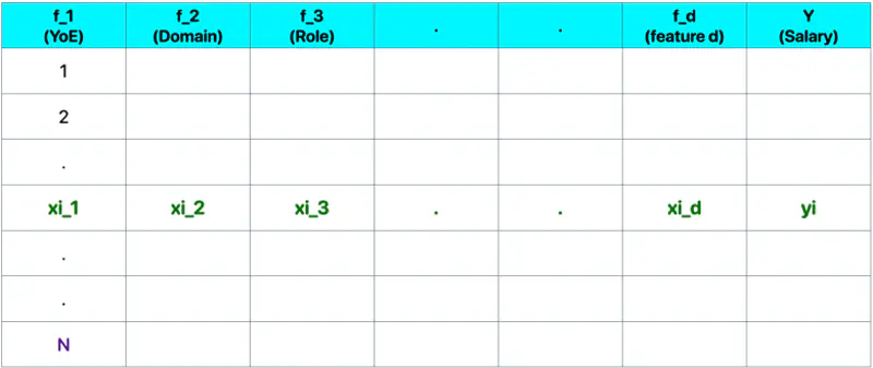
\[ \begin{align*} x_1 &= \text{Years of Experience} \\ x_2 &= \text{Domain (Tech, BFSI, Telecom, etc.)} \\ x_3 &= \text{Role (Dev, Tester, DevOps, ML, etc.)} \\ x_d &= d^{th} ~ feature \\ w_0 &= \text{Salary of 0 years experience} \\ \end{align*} \]Space = ’d’ features + 1 target variable = ’d+1’ dimensions
In a ’d+1’ dimensional space, we try to fit a ’d’ dimensional hyperplane.
Let, data = \( {(x_i, y_i)}_{i=1}^N ; ~ x_i \in R^d , y_i \in R^d\)
where, N = number of training samples.
Note: Fitting hyperplane (\(y = w_1x_1 + w_2x_2 + \dots + w_dx_d + w_0\)) is the model.
Objective : find the parameters/weights (\(w_0, w_1, w_2, \dots w_d \)) of the model.
\(\mathbf{w} = \begin{bmatrix} w_1 \\ w_2 \\ \vdots \\ w_d \end{bmatrix}_{\text{d x 1}}\)
\( \mathbf{x_i} = \begin{bmatrix} x_{i_1} \\ x_{i_2} \\ \vdots \\ x_{i_d} \end{bmatrix}_{\text{d x 1}} \)
\( \mathbf{y} = \begin{bmatrix} y_1 \\ y_2 \\ \vdots \\ y_i \\ \vdots \\ y_n \end{bmatrix}_{\text{n x 1}} \)
\( X =
\begin{bmatrix}
x_{11} & x_{12} & \cdots & x_{1d} \\
x_{21} & x_{22} & \cdots & x_{2d} \\
\vdots & \vdots & \ddots & \vdots \\
x_{i1} & x_{i2} & \cdots & x_{id} \\
\vdots & \vdots & \ddots & \vdots \\
x_{n1} & x_{n2} & \cdots & x_{nd} \\
\end{bmatrix}
_{\text{n x d}}
\)
Prediction:
Error = Actual - Predicted
\[ \epsilon_i = y_i - \hat{y_i}\]Goal : Minimize error between actual and predicted.
We can quantify the error for a single data point in following ways:
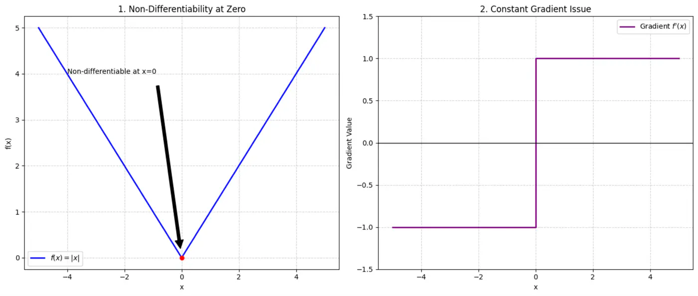
- Absolute error = \(|y_i - \hat{y_i}|\)
- Squared error = \((y_i - \hat{y_i})^2\)
Not differentiable at x=0, required for gradient descent.
Constant gradient, i.e \(\pm 1\), model learns at same rate, whether the error is large or small.
Average loss across all data points.
Mean Squared Error (MSE) =
\[ J(w) = \frac{1}{n} \sum_{i=1}^N (y_i - \hat{y_i})^2 \]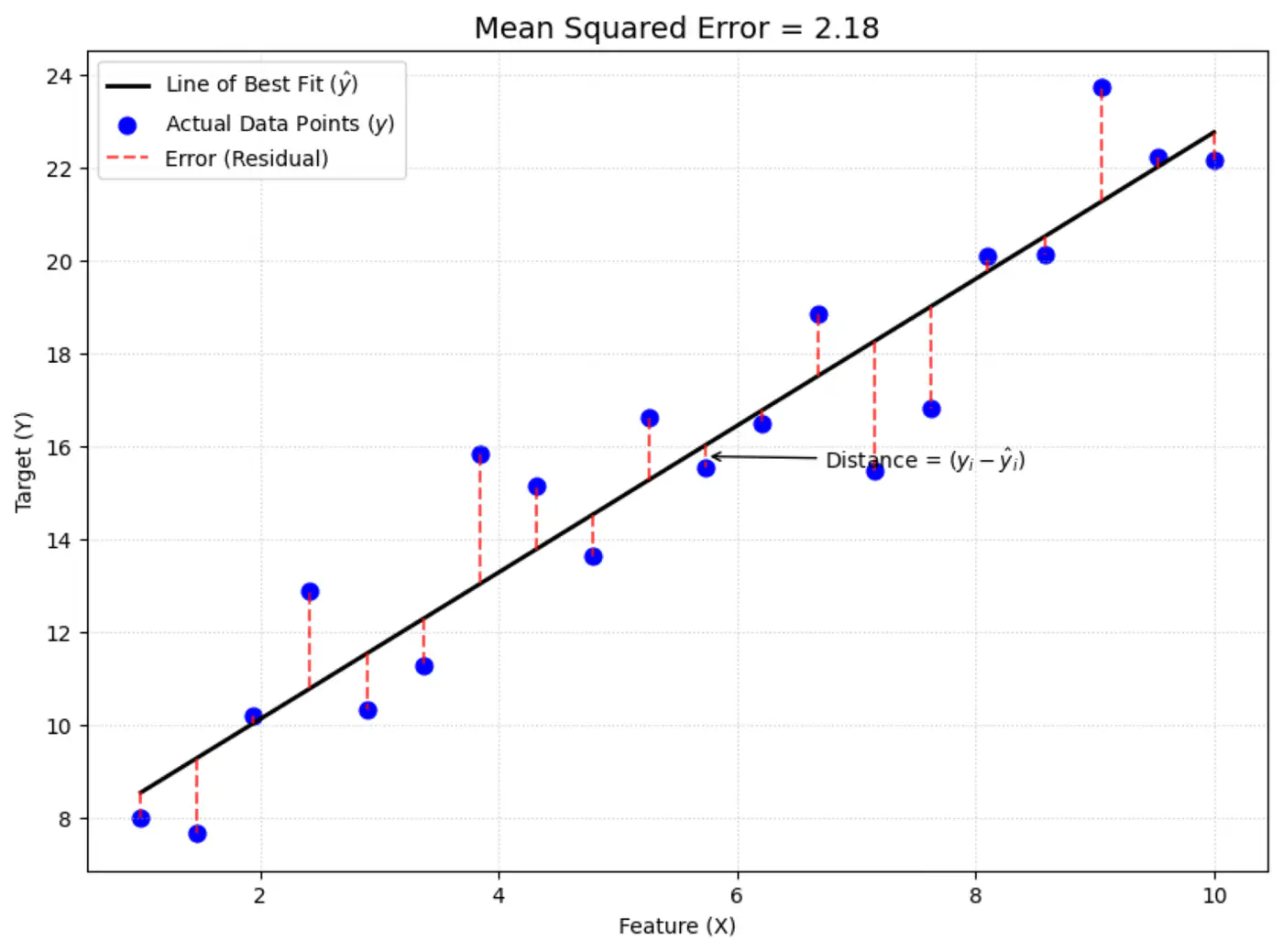
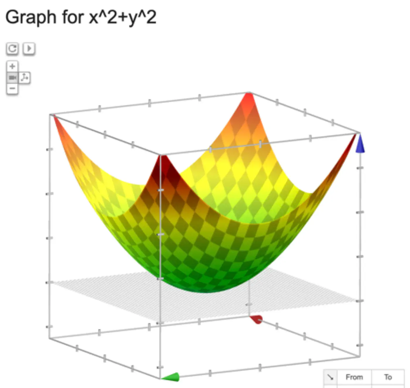
The above equation is quadratic in \(w_0, w_1, w_2, \dots w_d \).
Below is an image of a Paraboloid in 3D, similarly we will have a Paraboloid in ’d’ dimensions.
In order to find the minima of the cost function we need to take its derivative w.r.t weights and equate to 0.
\[ \begin{align*} \frac{\partial{J(w)}}{\partial{w_0}} = 0 \\ \frac{\partial{J(w)}}{\partial{w_1}} = 0 \\ \frac{\partial{J(w)}}{\partial{w_2}} = 0 \\ \vdots \\ \frac{\partial{J(w)}}{\partial{w_d}} = 0 \\ \end{align*} \]We have ‘d+1’ linear equations to solve for ‘d+1’ weights \(w_0, w_1, w_2, \dots , w_d\).
But solving ‘d+1’ system of linear equations (called the ’normal equations’) is tedious and NOT used for practical purposes.
where,
\(\mathbf{w} = \begin{bmatrix} w_1 \\ w_2 \\ \vdots \\ w_d \end{bmatrix}_{\text{d x 1}}\)
\( \mathbf{x_i} = \begin{bmatrix} x_{i_1} \\ x_{i_2} \\ \vdots \\ x_{i_d} \end{bmatrix}_{\text{d x 1}} \)
\( \mathbf{y} = \begin{bmatrix} y_1 \\ y_2 \\ \vdots \\ y_i \\ \vdots \\ y_n \end{bmatrix}_{\text{n x 1}} \)
\( X =
\begin{bmatrix}
x_{11} & x_{12} & \cdots & x_{1d} \\
x_{21} & x_{22} & \cdots & x_{2d} \\
\vdots & \vdots & \ddots & \vdots \\
x_{i1} & x_{i2} & \cdots & x_{id} \\
\vdots & \vdots & \ddots & \vdots \\
x_{n1} & x_{n2} & \cdots & x_{nd} \\
\end{bmatrix}
_{\text{n x d}}
\)
Prediction:
Let’s expand the cost function J(w):
\[ \begin{align*} J(w) &= \frac{1}{n} (y - Xw)^2 \\ &= \frac{1}{n} (y - Xw)^T(y - Xw) \\ &= \frac{1}{n} (y^T - w^TX^T)(y - Xw) \\ J(w) &= \frac{1}{n} (y^Ty - w^TX^Ty - y^TXw + w^TX^TXw) \end{align*} \]Since,\(w^TX^Ty\), is a scalar, so it is equal to its transpose.
\[ w^TX^Ty = (w^TX^Ty)^T = y^TXw\]\[ J(w) = \frac{1}{n} (y^Ty - y^TXw - y^TXw + w^TX^TXw)\]\[ J(w) = \frac{1}{n} (y^Ty - 2y^TXw + w^TX^TXw) \]Note: \(X^2 = X^TX\) and \((AB)^T = B^TA^T\)
To find the minimum, take the derivative of cost function J(w) w.r.t ‘w’, and equate to 0 vector.
\[\frac{\partial{J(w)}}{\partial{w}} = \vec{0}\]\[ \begin{align*} &\frac{\partial{[\frac{1}{n} (y^Ty - 2y^TXw + w^TX^TXw)]}}{\partial{w}} = 0\\ & \implies 0 - 2X^Ty + (X^TX + X^TX)w = 0 \\ & \implies \cancel{2}X^TXw = \cancel{2} X^Ty \\ & \therefore \mathbf{w} = (X^TX)^{-1}X^T\mathbf{y} \end{align*} \]Note: \(\frac{\partial{(a^T\mathbf{x})}}{\partial{\mathbf{x}}} = a\) and \(\frac{\partial{(\mathbf{x}^TA\mathbf{x})}}{\partial{\mathbf{x}}} = (A + A^T)\mathbf{x}\)
This is the closed-form solution of normal equations.
- Inverse may NOT exist (non-invertible).
- Time complexity of calculating the inverse is O(n^3).
If the inverse does NOT exist then we can use the approximation of the inverse, also called Pseudo Inverse or Moore Penrose Inverse (\(A^+\)).
Moore Penrose Inverse ( \(A^+\)) is calculated using Singular Value Decomposition (SVD).
SVD of \(A = U \Sigma V^T\)
Pseudo Inverse \(A^+ = V \Sigma^+ U^T\)
Where, \(\Sigma^+\) is a transpose of \(\Sigma\) with reciprocals of non-zero singular values on its diagonals.
e.g:
Note: Time Complexity = O(mn^2)