Probabilistic Interpretation
3 minute read
Error = Random Noise, Un-modeled effects
\[ \begin{align*} \epsilon_i = y_i - \hat{y_i} \\ \implies y_i = \hat{y_i} + \epsilon_i \\ \because \hat{y_i} = x_i^Tw \\ \therefore y_i = x_i^Tw + \epsilon_i \\ \end{align*} \]Actual value(\(y_i\)) = Deterministic linear predictor(\(x_i^Tw\)) + Error term(\(\epsilon_i\))
- Independent and Identically Distributed (I.I.D):
Each error term is independent of others. - Normal (Gaussian) Distributed:
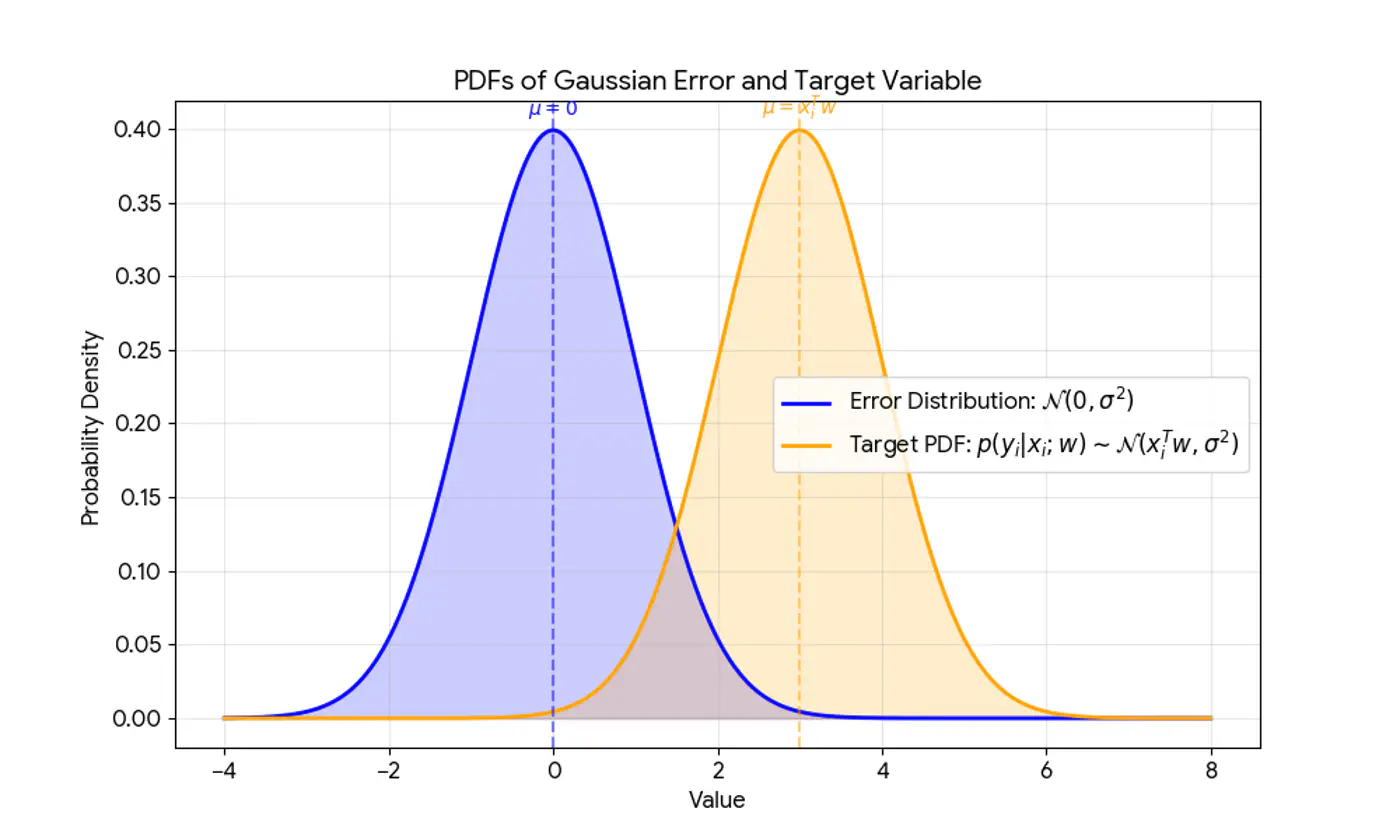
Error follows a normal distribution with mean = 0 and a constant variance, .
This implies that the target variable itself is a random variable, normally distributed around the linear relationship.
\[(y_{i}|x_{i};w)∼N(x_{i}^{T}w,\sigma^{2})\]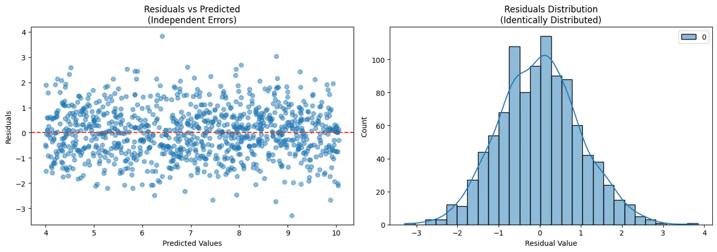
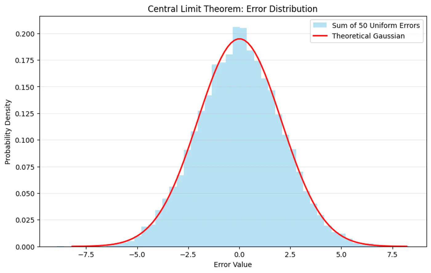
Central Limit Theorem (CLT) states that for a sequence of I.I.D random variables, the distribution of the sample mean(sum) approximates to a normal distribution, regardless of the original population distribution.
- Probability (Forward View):
Quantifies the chance of observing a specific outcome given a known, fixed model. - Likelihood (Backward/Inverse View):
Inverse concept used for inference (working backward from results to causes). It is a function of the parameters and measures how ‘likely’ a specific set of parameters makes the observed data appear.
‘Find the most plausible explanation for what I see.'
The goal of the probabilistic interpretation is to find the parameters ‘w’ that maximize the probability (likelihood) of observing the given dataset.
Assumption: Training data is I.I.D.
\[ \begin{align*} Likelihood &= \mathcal{L}(w) \\ \mathcal{L}(w) &= p(y|x;w) \\ &= \prod_{i=1}^N p(y_i| x_i; w) \\ &= \prod_{i=1}^N \frac{1}{\sigma\sqrt{2\pi}}e^{-\frac{(y_i-x_i^Tw)^2}{2\sigma^2}} \end{align*} \]Maximizing the likelihood function is mathematically complex due to the product term and the exponential function.
A common simplification is to maximize the log-likelihood function instead, which converts the product into a sum.
Note: Log is a strictly monotonically increasing function.
Note: The first term is constant w.r.t ‘w'.
So, we need to find parameters ‘w’ that maximize the log likelihood.
\[ \begin{align*} log \mathcal{L}(w) & \propto -\frac{1}{2\sigma^2} \sum_{i=1}^N (y_i-x_i^Tw)^2 \\ & \because \frac{1}{2\sigma^2} \text{ is constant} \\ log \mathcal{L}(w) & \propto -\sum_{i=1}^N (y_i-x_i^Tw)^2 \\ \end{align*} \]Maximizing the log-likelihood is equivalent to minimizing the sum of squared errors, which is the exact objective of the ordinary least squares (OLS) method.
\[ \underset{w}{\mathrm{min}}\ J(w) = \underset{w}{\mathrm{min}}\ \sum_{i=1}^N (y_i - x_i^Tw)^2 \]End of Section