Regularization
Regularization
3 minute read
Over-Fitting
Over-Fitting happens when we have a complex model that creates highly erratic curve to fit every single data point, including the random noise.
- Excellent performance on training 🏃♂️ data, but poor performance on unseen data.
How to Avoid Over-Fitting ?
- Penalty for overly complex models, i.e, models with excessively large or numerous parameters.
- Focus on learning general patterns rather than memorizing 🧠 everything, including noise in training 🏃♂️data.
Regularization
Set of techniques that prevents over-fitting by adding a penalty term to the model’s loss function.
\[ J_{reg}(w) = J(w) + \lambda.\text{Penalty(w)} \]\(\lambda\) = Regularization strength hyper parameter, bias-variance tradeoff knob.
- High \(\lambda\): High ⬆️ penalty, forces weights towards 0, simpler model.
- Low \(\lambda\): Weak ⬇️ penalty, closer to un-regularized model.
Regularization introduces Bias
- By intentionally simplifying a model (shrinking weights) to reduce its complexity, which prevents it from overfitting.
- Penalty pulls feature weights closer to zero, making the model less faithful representation of the training data’s true complexity.
Common Regularization Techniques
- L2 Regularization (Ridge Regression)
- L1 Regularization (Lasso Regression)
- Elastic Net Regularization
- Early Stopping
- Dropout (Neural Networks)
L2 Regularization
\[ \underset{w}{\mathrm{min}}\ J_{reg}(w) = \underset{w}{\mathrm{min}}\ \frac{1}{n} \sum_{i=1}^n (y_i - x_i^Tw)^2 + \lambda.\sum_{j=1}^n w_j^2 \]
- Penalty term: \(\ell_2\) norm - penalizes large weights quadratically.
- Pushes the weights close to 0 (not exactly 0), making models more stable by distributing importance across weights.
- Splits feature importance across co-related features.
- Use case: Best when most features are relevant and co-related.
- Also known as Ridge regression or Tikhonov regularization.
L1 Regularization
\[ \underset{w}{\mathrm{min}}\ J_{reg}(w) = \underset{w}{\mathrm{min}}\ \frac{1}{n} \sum_{i=1}^n (y_i - x_i^Tw)^2 + \lambda.\sum_{j=1}^n |w_j| \]
- Penalty term: \(\ell_1\) norm.
- Shrinks some weights exactly to 0, effectively performing feature selection, giving sparse solutions.
- For a group of highly co-related features, arbitrarily selects one feature and shrinks others to 0.
- Use case: Best when using high-dimensional datasets (d»n) where we suspect many features are irrelevant or redundant, or when model interpretability matters.
- Also known as Lasso (Least Absolute Shrinkage and Selection Operator) regression.
- Computational hack: \(\frac{\partial{|w_j|}}{\partial{w_j}} = 0\), since absolute function is not differentiable at 0.
Elastic Net Regularization
\[ \underset{w}{\mathrm{min}}\ J_{reg}(w) = \underset{w}{\mathrm{min}}\ \frac{1}{n} \sum_{i=1}^n (y_i - x_i^Tw)^2 + \lambda.((1-\alpha).\sum_{j=1}^n w_j^2 + \alpha.\sum_{j=1}^n |w_j|) \]
- Penalty term : linear combination of and norm.
- Sparsity(feature-selection) of L1 and stability/grouping effect of L2 regularization.
- Use case: Best when we have high dimensional data with correlated features and we want sparse and stable solution.
L1/L2/Elastic Net Regularization Comparison
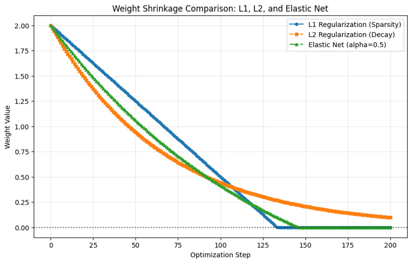
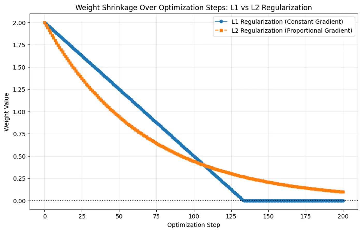
Question
Why weights shrink exactly to 0 in L1 regularization but NOT in L2 regularization ?
Answer
- Because the gradient of L1 penalty (absolute function) is a constant value, i.e, \(\pm 1\), this means a constant reduction in weight at each step, making it gradually reach to 0 in finite steps.
- Whereas, the derivative of L2 penalty is proportional to the weight (\(2w_j\)) and as the weight reaches close to 0, the gradient also becomes very small, this means that the weight will become very close to 0, but not exactly equal to 0.
L1 vs L2 Regularization Comparison
Video
Regularization (L1/L2/ElasticNet) | Why weights shrink to 0 in L1 Regularization ? | Explained
End of Section