Log Loss
Log Loss
3 minute read
Log Loss
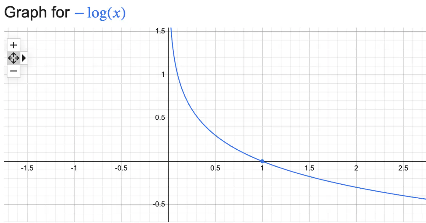
Log Loss = \(\begin{cases} -log(\hat{y_i}) & \text{if } y_i = 1 \\ \\ -log(1-\hat{y_i}) & \text{if } y_i = 0 \end{cases} \)
Combining the above 2 conditions into 1 equation gives:
Log Loss = \(-[y_ilog(\hat{y_i}) + (1-y_i)log(1-\hat{y_i})]\)
Cost Function
\[J(w) = -\frac{1}{n}\sum [y_ilog(\hat{y_i}) + (1-y_i)log(1-\hat{y_i})]\]
We need to find the weights 🏋️♀️ ‘w’ that minimize the cost 💵 function.
Gradient Descent
- Weight update: \[w_{new}=w_{old}-η.\frac{∂J(w)}{∂w_{old}}\]
We need to find the gradient of log loss w.r.t weight ‘w’.
Gradient Calculation
Chain Rule:
\[\frac{\partial{J(w)}}{\partial{w}} = \frac{\partial{J(w)}}{\partial{\hat{y}}}.\frac{\partial{\hat{y}}}{\partial{z}}.\frac{\partial{z}}{\partial{w}}\]- Cost Function: \(J(w) = -\frac{1}{n}\sum [y_ilog(\hat{y_i}) + (1-y_i)log(1-\hat{y_i})]\)
- Prediction: \(\hat{y} = \sigma(z) = \frac{1}{1 + e^{-z}}\)
- Distance of Point: \(z = \mathbf{w^Tx} + w_0\)
Cost 💰Function Derivative
\[ J(w) = -\sum [ylog(\hat{y}) + (1-y)log(1-\hat{y})]\]
How loss changes w.r.t prediction ?
\[ \begin{align*} \frac{\partial{J(w)}}{\partial{\hat{y}}} &= - [\frac{y}{\hat{y}} - \frac{1-y}{1-\hat{y}}] \\ &= -[\frac{y- \cancel{y\hat{y}} -\hat{y} + \cancel{y\hat{y}}}{\hat{y}(1-\hat{y})}] \\ \therefore \frac{\partial{J(w)}}{\partial{\hat{y}}} &= \frac{\hat{y} - y}{\hat{y}(1-\hat{y})} \end{align*} \]Prediction Derivative
\[ \hat{y} = \sigma(z) = \frac{1}{1 + e^{-z}} \]
How prediction changes w.r.t distance ?
\[ \begin{align*} \frac{\partial{\hat{y}}}{\partial{z}} &= \frac{\partial{\sigma(z)}}{\partial{z}} = \sigma'(z) \\ \sigma'(z) &= \sigma(z)(1-\sigma(z)) \\ \therefore \frac{\partial{\hat{y}}}{\partial{z}} &= \hat{y}(1-\hat{y}) \end{align*} \]Sigmoid Derivative
\[ \sigma(z) = \frac{1}{1 + e^{-z}} \]\[
\begin{align}
&\text {Let } u = 1 + e^{-z} \nonumber \\
&\implies \sigma(z) = \frac{1}{u}, \quad \text{so, } \nonumber \\
&\frac{\partial{\sigma(z)}}{\partial{z}} = \frac{\partial{\sigma(z)}}{\partial{u}}.
\frac{\partial{u}}{\partial{z}} \nonumber \\
&\frac{\partial{\sigma(z)}}{\partial{u}} = -\frac{1}{u^2} = - \frac{1}{(1 + e^{-z})^2} \\
&\text{and } \frac{\partial{u}}{\partial{z}} = \frac{\partial{(1 + e^{-z})}}{\partial{z}} = -e^{-z}
\end{align}
\]
from equations (1) & (2):
\[ \begin{align*} \because \frac{\partial{\sigma(z)}}{\partial{z}} &= \frac{\partial{\sigma(z)}}{\partial{u}}. \frac{\partial{u}}{\partial{z}} \\ \implies \frac{\partial{\sigma(z)}}{\partial{z}} &= - \frac{1}{(1 + e^{-z})^2}. -e^{-z} = \frac{e^{-z}}{(1 + e^{-z})^2} \\ 1 - \sigma(z) & = 1 - \frac{1}{1 + e^{-z}} = \frac{e^{-z}}{1 + e^{-z}} \\ \frac{\partial{\sigma(z)}}{\partial{z}} &= \frac{1}{1 + e^{-z}}.\frac{e^{-z}}{1 + e^{-z}} \\ \therefore \frac{\partial{\sigma(z)}}{\partial{z}} &= \sigma(z).(1-\sigma(z)) \end{align*} \]Distance Derivative
\[z=w^{T}x+w_{0}\]
How distance changes w.r.t weight 🏋️♀️ ?
\[ \frac{\partial{z}}{\partial{w}} = \mathbf{x} \]\[\because \frac{\partial{(a^T\mathbf{x})}}{\partial{\mathbf{x}}} = a\]Gradient Calculation (combined)
Chain Rule:
\[ \begin{align*} \frac{\partial{J(w)}}{\partial{w}} &= \frac{\partial{J(w)}}{\partial{\hat{y}}}.\frac{\partial{\hat{y}}}{\partial{z}}.\frac{\partial{z}}{\partial{w}} \\ &= \frac{\hat{y} - y}{\cancel{\hat{y}(1-\hat{y})}}.\cancel{\hat{y}(1-\hat{y})}.x \\ \therefore \frac{\partial{J(w)}}{\partial{w}} &= (\hat{y} - y).x \end{align*} \]Cost 💰Function Derivative
\[\frac{\partial{J(w)}}{\partial{w}} = \sum (\hat{y_i} - y_i).x_i\]
Gradient = Error x Input
- Error = \((\hat{y_i}-y_i)\): how far is prediction from the truth?
- Input = \(x_i\): contribution of specific feature to the error.
Gradient Descent (update)
Weight update:
\[w_{new} = w_{old} - \eta. \sum_{i=1}^n (\hat{y_i} - y_i).x_i\]Why MSE can NOT be used as Loss Function?
Mean Squared Error (MSE) can not be used to quantify error/loss in binary classification because:
- Convexity : MSE combined with Sigmoid is non-convex, so, Gradient Descent can get trapped in local minima.
- Penalty: MSE does not appropriately penalize mis-classifications in binary classification.
- e.g: If actual value is class 1 but the model predicts class 0, then MSE = \((1-0)^2 = 1\), which is very low, whereas log loss = \(-log(0) = \infty\)
End of Section