Kernel Trick
3 minute read
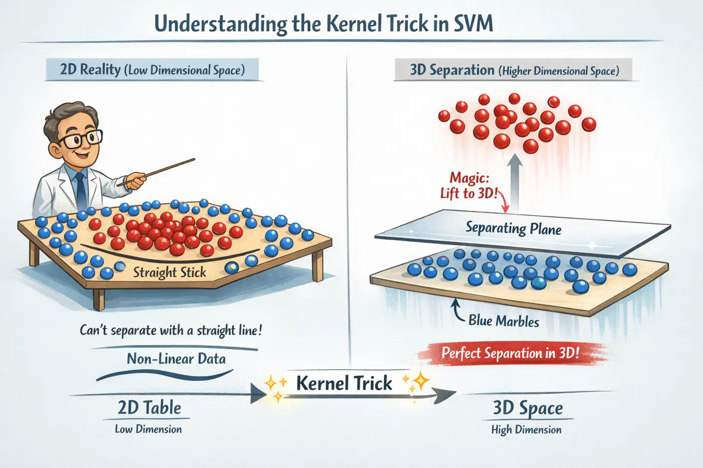
👉If our data is not linearly separable in its original space , we can map it to a higher-dimensional feature space (where D»d) using a transformation function .
- Bridge between Dual formulation and the geometry of high dimensional spaces.
- It is a way to manipulate inner product spaces without the computational cost 💰 of explicit transformation.
subject to: \(0 \leq \alpha_i \leq C\) and \(\sum \alpha_i y_i = 0\)
💡Actual values of the input vectors \(x_i\) and \(x_j\) never appear in isolation; only appear as inner product.
\[ \max_{\alpha} \sum_{i=1}^n \alpha_i - \frac{1}{2} \sum_{i,j=1}^n \alpha_i \alpha_j y_i y_j \mathbf{(x_i \cdot x_j)}\]\[f(x_q) = \text{sign}\left( \sum_{i=1}^n \alpha_i y_i (x_i^T x_q) + w_0 \right)\]👉The ‘shape’ of the decision boundary is entirely determined by how similar points are to one another, not by their absolute coordinates.
So we define a function called ‘Kernel Function’.
The ‘Kernel Trick’ 🪄 is an optimization that replaces the dot product of a high-dimensional mapping with a function of the dot product in the original space.
\[(x_i, x_j) = \langle \phi(x_i), \phi(x_j) \rangle\]💡How it works ?
Instead of mapping (to higher dimension) \(x_i \rightarrow \phi(x_i)\), \(x_j \rightarrow \phi(x_j)\),
and calculating the dot product.
We simply compute \(K(x_i, x_j)\) directly in the original input space.
👉The ‘Kernel Function’ gives the similar mathematical equivalent of mapping it to a higher dimensions and taking the dot product.
Note: For \(K(x_i, x_j)\) to be a valid kernel, it must satisfy Mercer’s Condition.
Below is an example for a quadratic Kernel function in 2D that is equivalent to mapping the vectors to 3D and taking a dot product in 3D.
\[K(x, z) = (x^T z)^2\]\[(x_1 z_1 + x_2 z_2)^2 = x_1^2 z_1^2 + 2x_1 z_1 x_2 z_2 + x_2^2 z_2^2\]The output of above quadratic kernel function is equivalent to the explicit dot product of two vectors in 3D:
\[\phi(x) = [x_1^2, \sqrt{2}x_1x_2, x_2^2]^T\]\[\phi(z) = [z_1^2, \sqrt{2}z_1z_2, z_2^2]^T\]\[\phi (x)\cdot \phi (z)=x_{1}^{2}z_{1}^{2}+2x_{1}x_{2}z_{1}z_{2}+x_{2}^{2}z_{2}^{2}\]- Computational Efficiency: Avoids the ‘combinatorial blowup’ 💥 of generating thousands of interaction features manually.
- Memory Savings: No need to store 💾 or process high-dimensional coordinates, only the scalar result of the kernel function.
- Designing special purpose domain specific kernel is very hard.
- Basically, we are trying to replace feature engineering with kernel design.
- Note: Deep learning does feature engineering implicitly for us.
- Runtime complexity depends on number of support vectors, whose count is not easy to control.
Note: Runtime Time Complexity ⏰ = \(O(n_{SV}\times d)\) , whereas linear SVM,\(O(d)\) .
End of Section