Elliptic Envelope
3 minute read
Detect anomalies in multivariate Gaussian data, such as, biometric data (height/weight) where features are normally distributed and correlated.
Assumption: The data can be modeled by a Gaussian distribution.
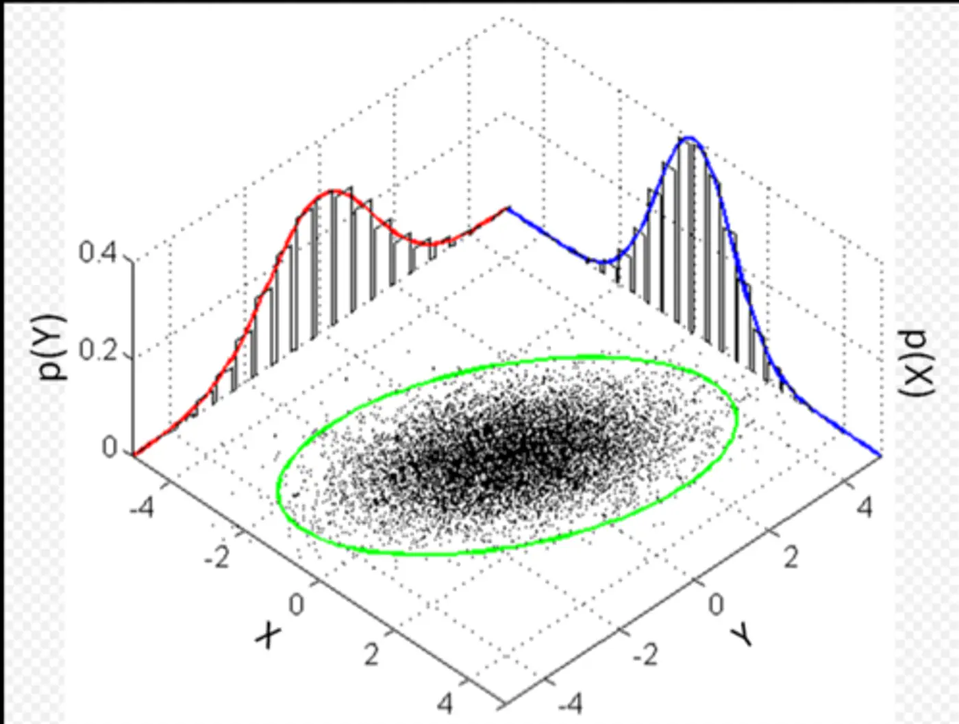
In a normal distribution, most data points cluster around the mean, and the probability density decreases as we move farther away from the center.
🌍 Euclidean distance measures the simple straight-line distance from the center of the cloud.
👉If the data is spherical, this works fine.
🦕 However, real-world data is often stretched or skewed (e.g., taller people are generally heavier), due to correlations between variables, forming an elliptical shape.
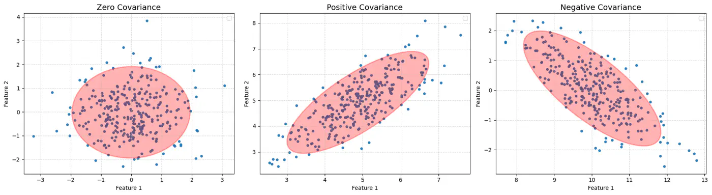
⭐️Mahalanobis distance essentially re-scales the data so that the elliptical distribution appears spherical, and then measures the Euclidean distance in that transformed space.
👉This way, it measures how many standard deviations(\(\sigma\)) away a point is from the mean, considering the data’s spread and correlation (covariance).
\[D_M(x) = \sqrt{(x - \mu)^T \Sigma^{-1} (x - \mu)}\]👉Find the most dense core of the data.
\[D_M(x) = \sqrt{(x - \mu)^T \Sigma^{-1} (x - \mu)}\]🦣 Determinant of covariance matrix \(\Sigma\) represents the volume of the ellipsoid.
⏲️ Therefore, minimize \(|\Sigma|\) to find the tight core.
👉 \(\text {Small} ~ \Sigma \rightarrow \text {Large} ~\Sigma ^{-1}\rightarrow \text {Large} ~ D_{M} ~\text {for outliers}\)
MCD algorithm is used to find the covariance matrix \(\Sigma\) with minimum determinant, so that the volume of the ellipsoid is minimized.
- Initialization: Select several random subsets of size h < n (default h = \(\frac{n+d+1}{2}\), d = # dimensions), representing ‘robust’ majority of the data.
- Calculate preliminary mean (\(\mu\)) and covariance (\(\Sigma\)) for each random subset.
- Concentration Step: Iterative core of the algorithm designed to ‘tighten’ the ellipsoid.
- Calculate Distances: Compute the Mahalanobis distance of all ’n’ points in the dataset from the current subset’s mean (\(\mu\)) and covariance (\(\Sigma\)).
- Select New Subset: Identify the ‘h’ points with the smallest Mahalanobis distances.
- These are the points most centrally located relative to the current ellipsoid.
- Update Estimates: Calculate a new and based only on these ‘h’ most central points.
- Repeat 🔁: The steps repeat until the determinant stops shrinking.
Note: Select the best subset that achieved the absolute minimum determinant.
- Assumptions
- Gaussian data.
- Unimodal data (single center).
- Cost 💰of covariance matrix \(\Sigma^{-1}\) inversion is O(d^3).
End of Section