Isolation Forest

‘Large scale tabular data.’

Credit card fraud detection in datasets with millions of rows and hundreds of features.

Note: Supervised learning requires balanced, labeled datasets (normal vs. anomaly), which are rarely available in real-world scenarios like fraud or cyber-attacks.

🦥 ‘Flip the logic.’

🦄 ‘Anomalies’ are few and different, so they are much easier to isolate from the rest of the data than normal points.

🐦‍🔥 ‘Curse of dimensionality.’

🐎 Distance based (K-NN), and density based (LOF) algorithms require calculation of distance between all pair of points.

🐙 As the number of dimensions and data points grows, these calculations become exponentially more expensive 💰 and less effective.

‘Randomly partition the data.’

🦄 If a point is an outlier, it will take fewer partitions (splits) to isolate it into a leaf 🍃 node compared to a point that is buried deep within a dense cluster of normal data.

🌳Isolation Forest uses an ensemble of ‘Isolation Trees’ (iTrees) 🌲.

👉iTree (Isolation Tree) 🌲 is a proper binary tree structure specifically designed to separate individual data points through random recursive partitioning.

1. Sub-sampling:
   • Select a random subset of data (typically 256 instances) to build an iTree.
2. Tree Construction: Randomly select a feature.
   • Randomly select a split value between the minimum and maximum values of that feature.
   • Divide the data into two branches based on this split.
   • Repeat recursively until the point is isolated or a height limit is reached.
3. Forest Creation:
   • Repeat 🔁 the process to create ‘N’ trees (typically 100).
4. Inference:
   • Pass a new data point through all trees, calculate the average path length, and compute the anomaly score.

⭐️🦄 Assign an anomaly score based on the path length h(x) required to isolate a point ‘x’.

• Path Length (h(x)): The number of edges ‘x’ traverses from the root node to a leaf node.
• Average Path Length (c(n)): Since iTrees are structurally similar to Binary Search Trees (BST), the average path length for a dataset of size ’n’ is given by: \[c(n)=2H(n-1)-\frac{2(n-1)}{n}\]

where, H(i) is the harmonic number, estimated as \(\ln (i)+0.5772156649\) (Euler’s constant).

To normalize the score between 0 and 1, we define it as:

👉E(H(x)): is the average path length of across a forest of trees 🌲.

• \(s\rightarrow 1\): Point is an anomaly; Path length is very short.
• \(s\approx 0.5\): Point is normal, path length approximately equal to c(n).
• \(s\rightarrow 0\): Point is normal; deeply buried point, path length is much larger than c(n).

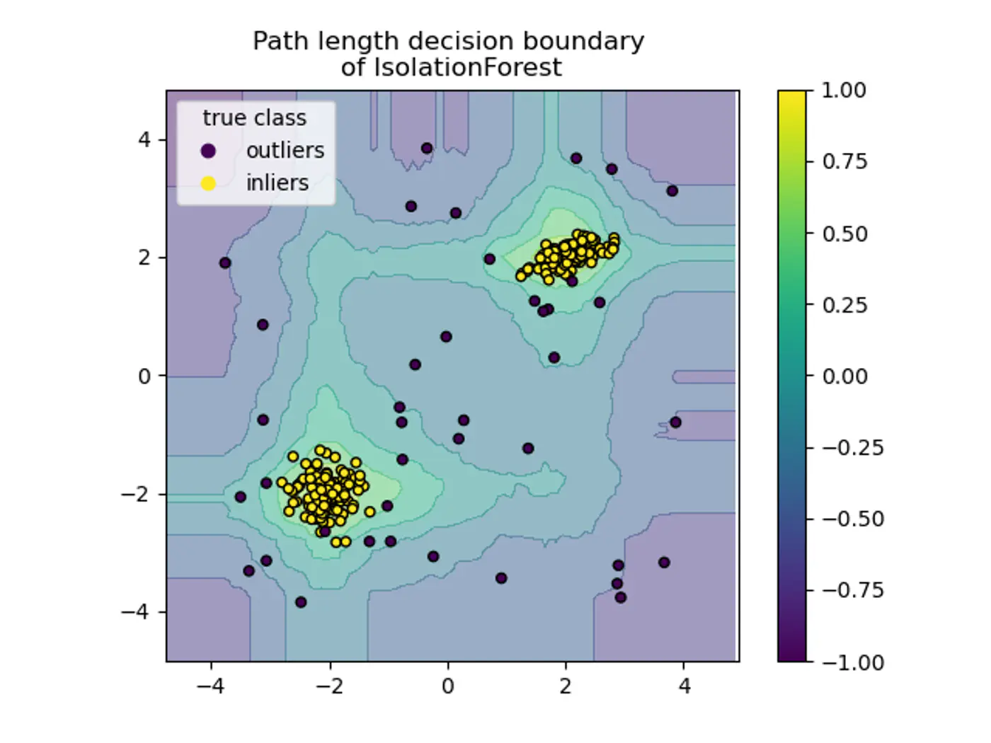
• Axis-Parallel Splits:
  • Standard iTrees 🌲 split only on one feature at a time, so:
    • We do not get a smooth decision boundary.
    • Anything off-axis has a higher probability of being marked as an outlier.
    • Note: Extended Isolation Forest fixes this by using random slopes.
• Score Sensitivity: The threshold for what constitutes an ‘anomaly’ often requires manual tuning or domain knowledge.