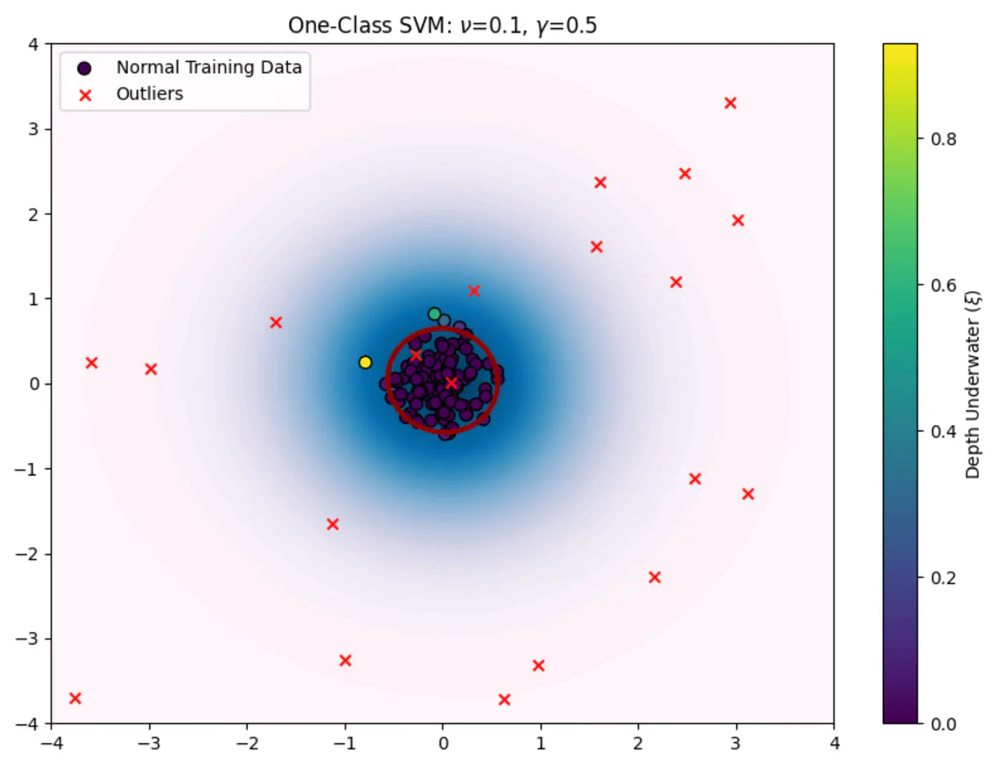
One Class SVM
3 minute read
⭐️Only one class of data (normal, non-outlier) is available for training, making standard supervised learning models impossible.
e.g. Only normal observations are available for fraud detection, cyber attack, fault detection etc.

🦂 The core problem is to build a model that can distinguish between ‘normal’ and ‘anomalous’ data when we only have examples of the ‘normal’ class during training.
🦖 We need to find a decision boundary that is as compact as possible while still encompassing the bulk of the training data.
🦍 Define a boundary for a single class in high-dimensional space where data might be non-linearly distributed (e.g.‘U’ shape).
🦧 Use the Kernel Trick to project data into a higher-dimensional space and find a hyperplane that separates the data from the origin with the maximum margin.
⭐️OC-SVM, as introduced by Bernhard Schölkopf et al., uses a hyperplane ‘H’ defined by a weight vector \(\mathbf{w}\) and a bias term \(\rho\).
👉Solve the following optimization problem:
\[\min _{\mathbf{w},\xi _{i},\rho }\frac{1}{2}||\mathbf{w}||^{2}+\frac{1}{\nu N}\sum _{i=1}^{N}\xi _{i}-\rho \]Subject to constraints:
\[\mathbf{w}\cdot \phi (\mathbf{x}_{i})\ge \rho -\xi _{i}\quad \text{and}\quad \xi _{i}\ge 0,\quad \text{for\ }i=1,\dots ,N\]- \(\mathbf{x}_{i}\): i-th training data point.
- \(\phi (\mathbf{x}_{i})\): RBF kernel function \(K(x, y) = \exp(-\gamma \|x-y\|^2)\) that maps the data into a higher-dimensional feature space, making it easier to separate from the origin.
- \(\mathbf{w}\): normal vector to the separating hyperplane.
- \(\rho\): scalar bias term that determines the offset of the hyperplane from the origin.
- \(\xi_i\): Slack variables that allow some data points to fall on the ‘wrong’ side of the hyperplane (inside the anomalous region) to prevent overfitting.
- N: total number of training points.
- \(\nu\): hyper-parameter between 0 and 1. It acts as an upper bound on the fraction of outliers (training data points outside the boundary) and a lower bound on the fraction of support vectors.
- \(\frac{1}{2}\|\mathbf{w}\|^{2}\): aims to maximize the margin/compactness of the region.
- \(\frac{1}{\nu N}\sum _{i=1}^{N}\xi _{i}-\rho\): penalizes points (outliers) that violate the boundary constraints.
After solving the optimization problem using standard quadratic programming techniques, we obtain the optimal \(\mathbf{w}^{*}\) and \(\rho ^{*}\).
For a new data point \(x_{new}\), decision function is:
\[f(\mathbf{x}_{\text{new}})=\text{sign}(\mathbf{w}^{*}\cdot \phi (\mathbf{x}_{\text{new}})-\rho ^{*})\]\(f(\mathbf{x}_{\text{new}})\ge 0\): normal point.
\(f(\mathbf{x}_{\text{new}})< 0\): anomalous point (outlier).

End of Section