t-SNE
4 minute read
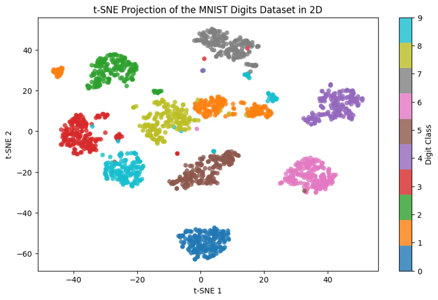
PCA preserves variance, not neighborhoods.
t-SNE focuses on the ‘neighborhood’ (local structure).
Tries to keep points that are close together in high-dimensional space close together in low-dimensional space.
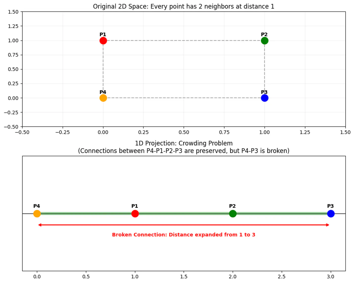
Map high-dimensional points to low-dimensional points , such that the pairwise similarities are preserved, while solving the ‘crowding problem’ (where points collapse into a single cluster).
Crowding Problem
Convert Euclidean distances into conditional probabilities representing similarities.
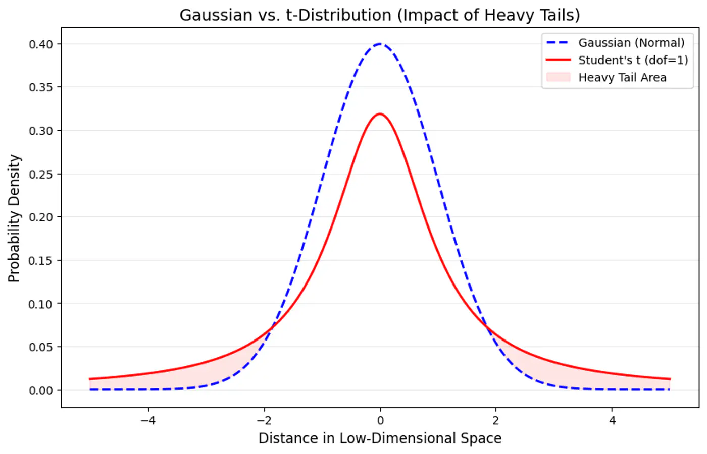
Minimize the divergence between the probability distributions of the high-dimensional (Gaussian) and low-dimensional (t-distribution) spaces.
Note: Probabilistic approach to defining neighbors is the core ‘stochastic’ element of the algorithm’s name.
The similarity of datapoint \(x_j\) to datapoint \(x_i\) is the conditional probability \(p_{j|i}\), that \(x_i\) would pick \(x_j\) as its neighbor.
Note: If neighbors are picked in proportion to their probability density under a Gaussian centered at \(x_i\).
\[p_{j|i} = \frac{\exp(-||x_i - x_j||^2 / 2\sigma_i^2)}{\sum_{k \neq i} \exp(-||x_i - x_k||^2 / 2\sigma_i^2)}\]- \(p_{j|i}\) high: nearby points.
- \(p_{j|i}\) low: widely separated points.
Note: Make probabilities symmetric: \(p_{ij} = \frac{p_{j|i} + p_{i|j}}{2n}\)
To solve the crowding problem, we use a heavy-tailed distribution (Student’s-t distribution with degree of freedom \(\nu=1\)).
\[q_{ij} = \frac{(1 + ||y_i - y_j||^2)^{-1}}{\sum_{k \neq l} (1 + ||y_k - y_l||^2)^{-1}}\]Note: Heavier tail spreads out dissimilar points more effectively, allowing moderately distant points to be mapped further apart, preventing clusters from collapsing and ensuring visual separation and cluster distinctness.
Measure the difference between the distributions ‘p’ and ‘q’ using the Kullback-Leibler (KL) divergence, which we aim to minimize:
\[C = KL(P||Q) = \sum_i \sum_j p_{ij} \log \frac{p_{ij}}{q_{ij}}\]Use gradient descent to iteratively adjust the positions of the low-dimensional points \(y_i\).
The gradient of the KL divergence is:
\[\frac{\partial C}{\partial y_{i}}=4\sum _{j\ne i}(p_{ij}-q_{ij})(y_{i}-y_{j})(1+||y_{i}-y_{j}||^{2})^{-1}\]- C : t-SNE cost function (sum of all KL divergences).
- \(y_i, y_j\): coordinates of data points and in the low-dimensional space (typically 2D or 3D).
- \(p_{ij}\): high-dimensional similarity (joint probability) between points \(x_i\) and \(x_j\), calculated using a Gaussian distribution.
- \(q_{ij}\): low-dimensional similarity (joint probability) between points \(y_i\) and \(y_j\), calculated using a Student’s t-distribution with one degree of freedom.
- \((1+||y_{i}-y_{j}||^{2})^{-1}\): term comes from the heavy-tailed Student’s t-distribution, which helps mitigate the ‘crowding problem’ by allowing points that are moderately far apart to have a small attractive force.
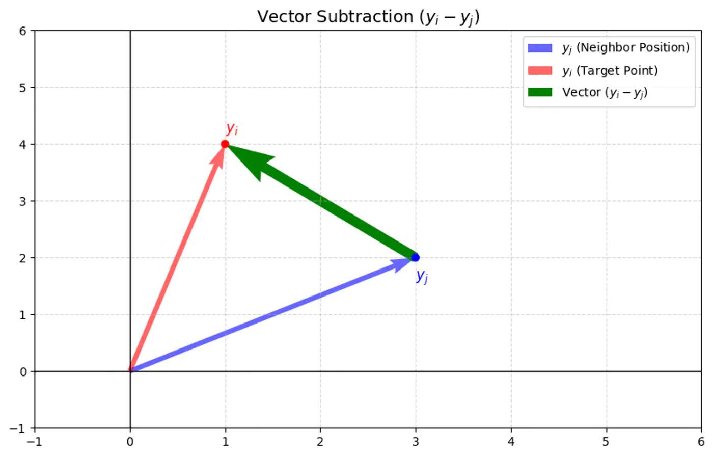
The gradient can be understood as a force acting on each point \(y_i\) in the low-dimensional map:
\[\frac{\partial C}{\partial y_{i}}=4\sum _{j\ne i}(p_{ij}-q_{ij})(y_{i}-y_{j})(1+||y_{i}-y_{j}||^{2})^{-1}\]- Attractive forces: If \(p_{ij}\) is large ⬆️ and \(q_{ij}\) is small ⬇️ (meaning two points were close in the high-dimensional space but are far in the low-dimensional space), the term \((p_{ij}-q_{ij})\) is positive, resulting in a strong attractive force pulling \(y_i\) and \(y_j\) closer.
- Repulsive forces: If \(p_{ij}\) is small ⬇️ and \(q_{ij}\) is large ⬆️ (meaning two points were far in the high-dimensional space but are close in the low-dimensional space), the term \((p_{ij}-q_{ij})\) is negative, resulting in a repulsive force pushing \(y_i\) and \(y_j\) apart.
Update step of in low dimensions:
\[y_{i}^{(t+1)}=y_{i}^{(t)}-\eta \frac{\partial C}{\partial y_{i}}\]Attractive forces (\(p_{ij}>q_{ij}\)):
- The negative gradient moves \(y_i\) opposite to the (\(y_i - y_j\)) vector, pulling it toward \(y_j\).
Repulsive forces (\(p_{ij} < q_{ij}\)):
- The negative gradient moves \(y_i\) in the same direction as the (\(y_i - y_j\)) vector, pushing it away from \(y_j\).
User-defined parameter that loosely relates to the effective number of neighbors.
Note: Variance \(\sigma_i^2\) (Gaussian) is adjusted for each point to maintain a consistent perplexity.