UMAP
3 minute read
🐢Visualizing massive datasets where t-SNE is too slow.
⭐️ Creating robust low-dimensional inputs for subsequent machine learning models.
⭐️ Using a world map 🗺️ (2D)instead of globe 🌍 for spherical(3D) earth 🌏.
👉It preserves the neighborhood relationships of countries (e.g., India is next to China), and to a good degree, the global structure.
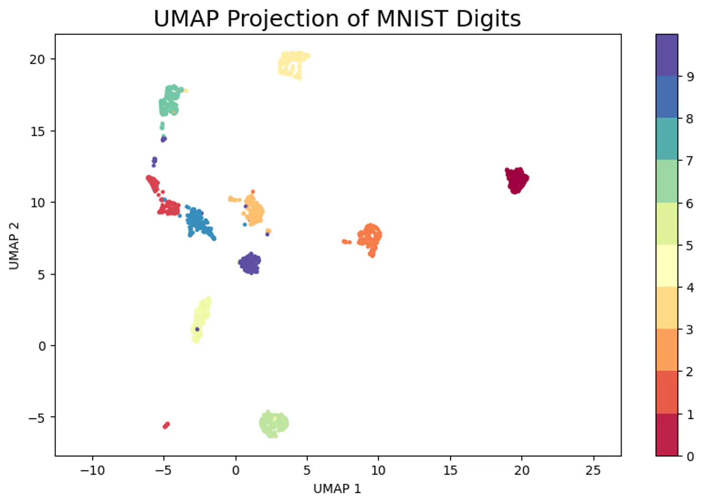
⭐️ Non-linear dimensionality reduction technique to visualize high-dimensional data (like images, gene expressions)
in a lower-dimensional space (typically 2D or 3D), preserving its underlying structure and relationships.
👉 Constructs a high-dimensional graph of data points and then optimizes a lower-dimensional layout to closely match this graph, making complex datasets understandable by revealing patterns, clusters, and anomalies.
Note: Similar to t-SNE but often faster and better at maintaining global structure.
💡 Create a weighted graph (fuzzy simplicial set) representing the data’s topology and then find a low-dimensional graph that is as structurally similar as possible.
Note: Fuzzy means instead of using binary 0/1, we use weights in the range [0,1] for each edge.
- UMAP determines local connectivity based on a user-defined number of neighbors (n_neighbors).
- Normalizes distances locally using the distance to the nearest neighbor (\(\rho_i\)) and a scaling factor (\(\sigma_i\)) adjusted to enforce local connectivity constraints.
- The weight \(W_{ij}\) (fuzzy similarity) in high-dimensional space is: \[W_{ij}=\exp \left(-\frac{\max (0,\|x_{i}-x_{j}\|-\rho _{i})}{\sigma _{i}}\right)\]
Note: This ensures that the closest point always gets a weight of 1, preserving local structure.
👉In the low-dimensional space (e.g., 2D), UMAP uses a simple curve (similar to the t-distribution used in t-SNE) for edge weights:
\[Z_{ij}=(1+a\|y_{i}-y_{j}\|^{2b})^{-1}\]Note: The parameters ‘a’ and ‘b’ are typically fixed based on the ‘min_dist’ user parameter (e.g. min_dist = 0.1, then a≈1,577, b≈0.895).
⭐️ Unlike t-SNE’s KL divergence, UMAP minimizes the cross-entropy between the high-dimensional weights \(W_{ij}\) and the low-dimensional weights \(Z_{ij}\).
👉 Cost 💰 Function (C):
\[C=\sum _{i,j}\left(W_{ij}\log \frac{W_{ij}}{Z_{ij}}+(1-W_{ij})\log \frac{1-W_{ij}}{1-Z_{ij}}\right)\]Cost 💰 Function (C):
\[C=\sum _{i,j}\left(W_{ij}\log \frac{W_{ij}}{Z_{ij}}+(1-W_{ij})\log \frac{1-W_{ij}}{1-Z_{ij}}\right)\]🎯 Goal : Reduce overall Cross Entropy Loss.
- Attractive Force: \(W_{ij}\) high; make \(Z_{ij}\) high to make the log \(\frac{W_{ij}}{Z_{ij}} \)term small.
- Repulsive Force: \(W_{ij}\) low; make \(Z_{ij}\) low to make the \(log\frac{1-W_{ij}}{1-Z_{ij}}\) term small.
Note: This push and pull of 2 ‘forces’ will make the data in low dimensions settle into a position that is overall a good representation of the original data in higher dimensions.
- Mathematically complex.
- Requires tuning (n_neighbors, min_dist).
End of Section