Latent Variable Model
4 minute read
⭐️Probabilistic model that assumes data is generated from a mixture of several Gaussian (normal) distributions with unknown parameters.
🎯GMM represents the probability density function of the data as a weighted sum of ‘K’ component Gaussian densities.
👉Below plot shows the probability of a point being generated by 3 different Gaussians.
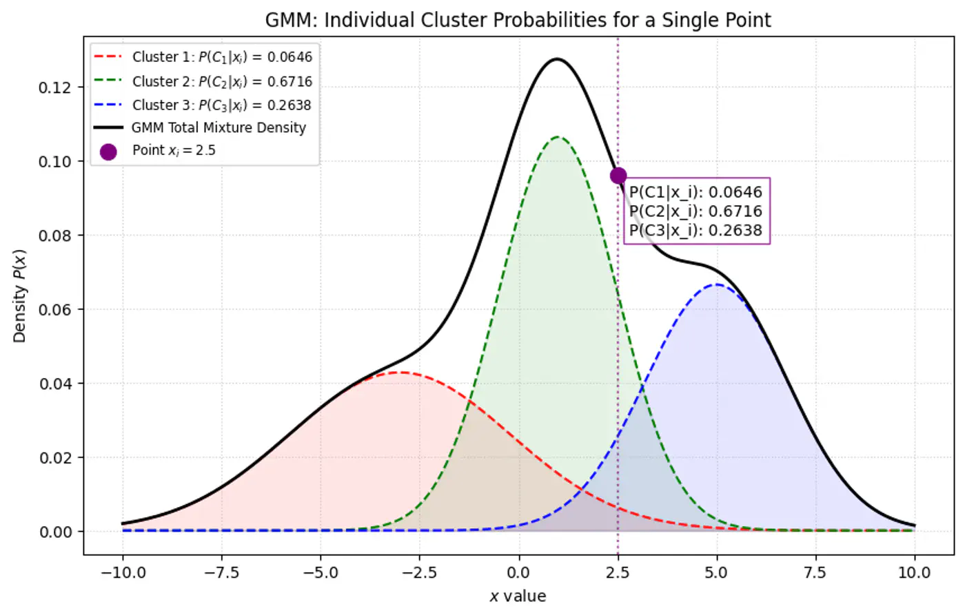
Overall density \(p(x_i|\mathbf{\theta })\) for a data point ‘\(x_i\)’:
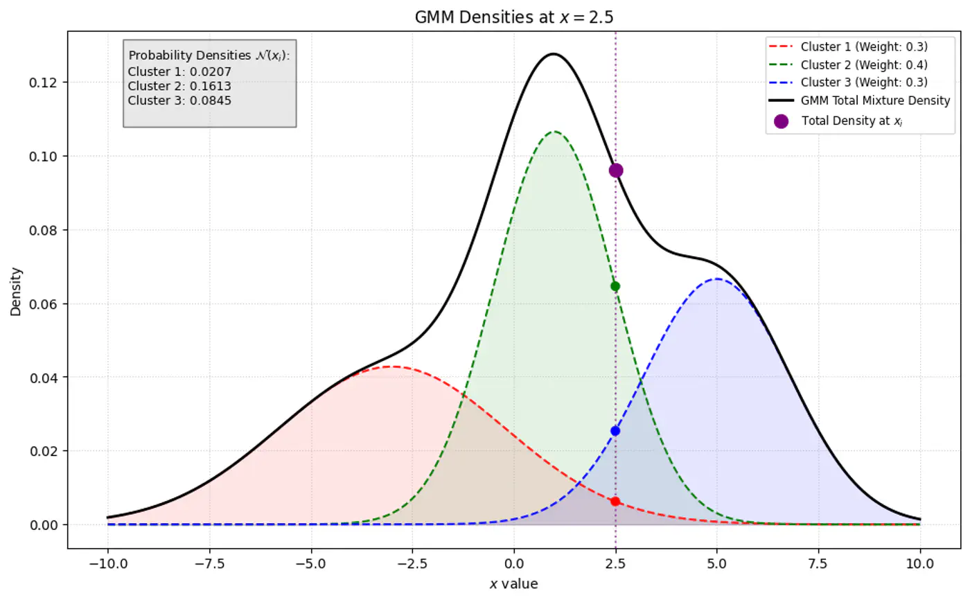
\[p(x_i|\mathbf{\mu},\mathbf{\Sigma} )=\sum _{k=1}^{K}\pi _{k}\mathcal{N}(x_i|\mathbf{\mu }_{k},\mathbf{\Sigma }_{k})\]- K: number of component Gaussians.
- \(\pi_k\): mixing coefficient (weight) of the k-th component, such that, \(\pi_k \ge 0\) and \(\sum _{k=1}^{K}\pi _{k}=1\).
- \(\mathcal{N}(x_i|\mathbf{\mu }_{k},\mathbf{\Sigma }_{k})\): probability density function of the k-th Gaussian component with mean \(\mu_k\) and covariance matrix \(\Sigma_k\).
- \(\mathbf{\theta }=\{(\pi _{k},\mathbf{\mu }_{k},\mathbf{\Sigma }_{k})\}_{k=1}^{K}\): complete set of parameters to be estimated.
Note: \(\pi _{k}\approx \frac{\text{Number\ of\ points\ in\ cluster\ }k}{\text{Total\ number\ of\ points\ }(N)}\)
👉 Weight of the cluster is proportional to the number of points in the cluster.
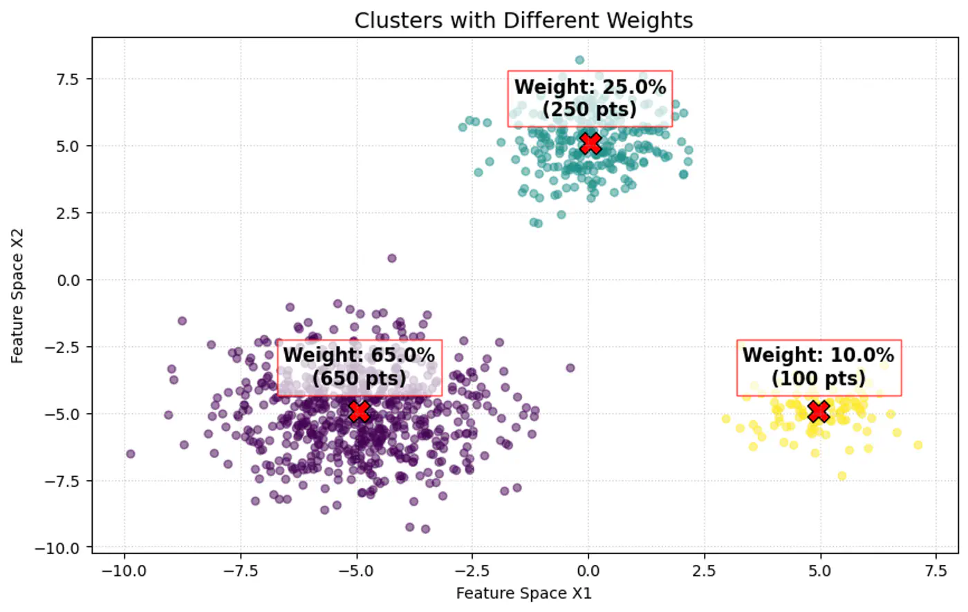
👉Below image shows the weighted Gaussian PDF, given the weights of clusters.
🎯 Goal of a GMM optimization is to find the set of parameters \(\Theta =\{(\pi _{k},\mu _{k},\Sigma _{k})\mid k=1,\dots ,K\}\) that maximize the likelihood of observing the given data.
\[L(\Theta |X)=\sum _{i=1}^{N}\log P(x_i|\Theta )=\sum _{i=1}^{N}\log \left(\sum _{k=1}^{K}\pi _{k}\mathcal{N}(x_i|\mu _{k},\Sigma _{k})\right)\]- 🦀 \(\log (A+B)\) cannot be simplified.
- 🦉So, is there any other way ?
⭐️Imagine we are measuring the heights of people in a college.
- We see a distribution with two peaks (bimodal).
- We suspect there are two underlying groups:
- Group A (Men) and Group B (Women).
Observation:
- Observed Variable (X): Actual height measurements.
- Latent Variable (Z): The ‘label’ (Man or Woman) for each person.
Note: We did not record gender, so it is ‘hidden’ or ‘latent’.
⭐️GMM is a latent variable model, meaning each data point \(\mathbf{x}_{i}\) is assumed to have an associated unobserved (latent) variable \(z_{i}\in \{1,\dots ,K\}\) indicating which component generated it.
Note: We observe the data point, but we do not observe which cluster it belongs to (\(z_i\)).
👉If we knew the value of \(z_i\) (component indicator) for every point, estimating the parameters of each Gaussian component would be straightforward.
Note: The challenge lies in estimating both the parameters of the Gaussians and the values of the latent variables simultaneously.
- With ‘z’ unknown:
- maximize: \[ \log \sum _{k}\pi _{k}\mathcal{N}(x_{i}|\mu _{k},\Sigma _{k}) = \log \Big(\pi _{1}\mathcal{N}(x_{i}\mid \mu _{1},\Sigma _{1})+\pi _{2}\mathcal{N}(x_{i}\mid \mu _{2},\Sigma _{2})+ \dots + \pi _{k}\mathcal{N}(x_{i}\mid \mu _{k},\Sigma _{k})\Big)\]
- \(\log (A+B)\) cannot be simplified.
- maximize: \[ \log \sum _{k}\pi _{k}\mathcal{N}(x_{i}|\mu _{k},\Sigma _{k}) = \log \Big(\pi _{1}\mathcal{N}(x_{i}\mid \mu _{1},\Sigma _{1})+\pi _{2}\mathcal{N}(x_{i}\mid \mu _{2},\Sigma _{2})+ \dots + \pi _{k}\mathcal{N}(x_{i}\mid \mu _{k},\Sigma _{k})\Big)\]
- With ‘z’ known:
- The log-likelihood of the ‘complete data’ simplifies into a sum of logarithms:
\[\sum _{i}\log (\pi _{z_{i}}\mathcal{N}(x_{i}|\mu _{z_{i}},\Sigma _{z_{i}}))\]
- Every point is assigned to exactly one cluster, so the sum disappears because there is only one cluster responsible for that point.
- The log-likelihood of the ‘complete data’ simplifies into a sum of logarithms:
\[\sum _{i}\log (\pi _{z_{i}}\mathcal{N}(x_{i}|\mu _{z_{i}},\Sigma _{z_{i}}))\]
Note: This allows the logarithm to act directly on the exponential term of the Gaussian, leading to simple linear equations.
👉When ‘z’ is known, every data point is ‘labeled’ with its parent component.
To estimate the parameters (mean \(\mu_k\) and covariance \(\Sigma_k\)) for a specific component ‘k’ :
- Gather all data points \(x_i\), where \(z_i\)= k.
- Calculate the standard Maximum Likelihood Estimate.(MLE) for that single Gaussian using only those points.
⭐️ Knowing ‘z’ provides exact counts and component assignments, leading to direct formulae for the parameters:
- Mean (\(\mu_k\)): Arithmetic average of all points assigned to component ‘k’.
- Covariance (\(\Sigma_k\)): Sample covariance of all points assigned to component ‘k’.
- Mixing Weight (\(\pi_k\)): Fraction of total points assigned to component ‘k’.
End of Section