Latent Variable Model
4 minute read
Probabilistic model that assumes data is generated from a mixture of several Gaussian (normal) distributions with unknown parameters.
GMM represents the probability density function of the data as a weighted sum of ‘K’ component Gaussian densities.
Below plot shows the probability of a point being generated by 3 different Gaussians.
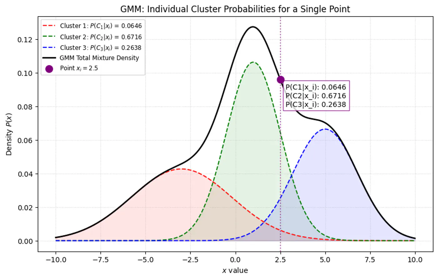
Overall density \(p(x_i|\mathbf{\theta })\) for a data point ‘\(x_i\)’:
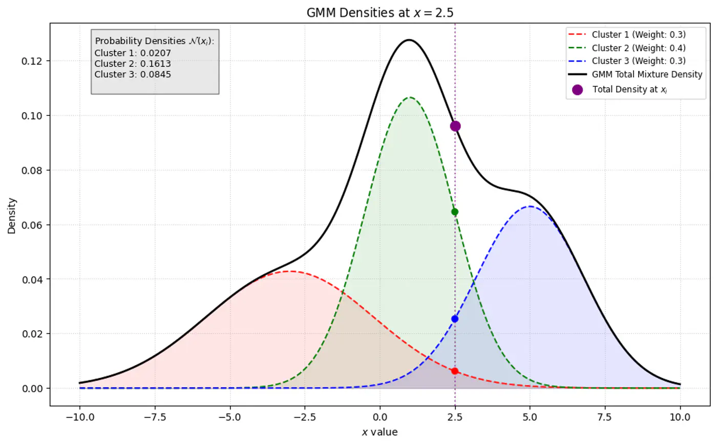
\[p(x_i|\mathbf{\mu},\mathbf{\Sigma} )=\sum _{k=1}^{K}\pi _{k}\mathcal{N}(x_i|\mathbf{\mu }_{k},\mathbf{\Sigma }_{k})\]- K: number of component Gaussians.
- \(\pi_k\): mixing coefficient (weight) of the k-th component, such that, \(\pi_k \ge 0\) and \(\sum _{k=1}^{K}\pi _{k}=1\).
- \(\mathcal{N}(x_i|\mathbf{\mu }_{k},\mathbf{\Sigma }_{k})\): probability density function of the k-th Gaussian component with mean \(\mu_k\) and covariance matrix \(\Sigma_k\).
- \(\mathbf{\theta }=\{(\pi _{k},\mathbf{\mu }_{k},\mathbf{\Sigma }_{k})\}_{k=1}^{K}\): complete set of parameters to be estimated.
Note: \(\pi _{k}\approx \frac{\text{Number\ of\ points\ in\ cluster\ }k}{\text{Total\ number\ of\ points\ }(N)}\)
Weight of the cluster is proportional to the number of points in the cluster.
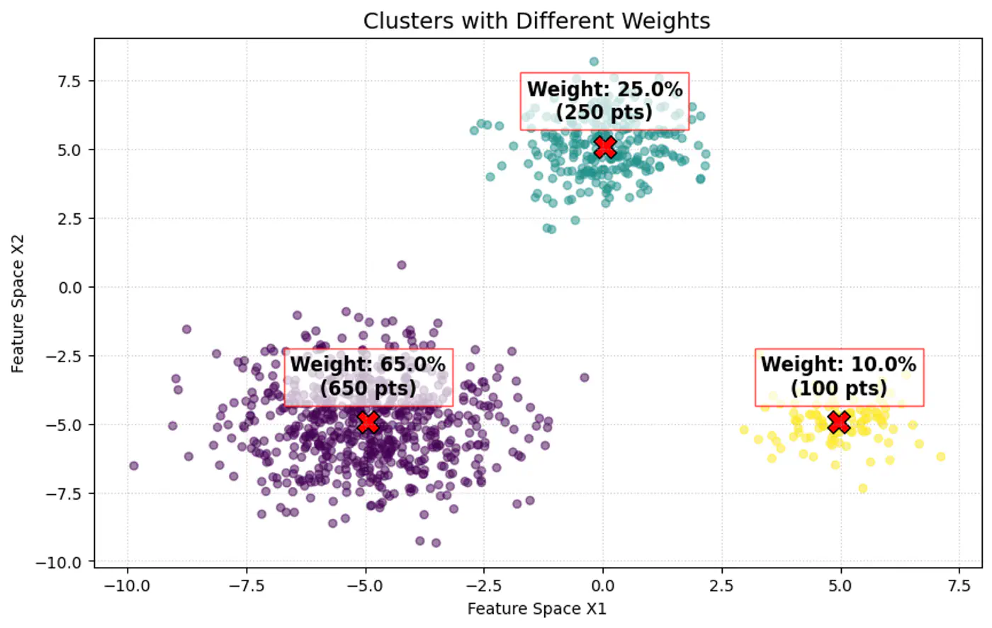
Below image shows the weighted Gaussian PDF, given the weights of clusters.
Goal of a GMM optimization is to find the set of parameters \(\Theta =\{(\pi _{k},\mu _{k},\Sigma _{k})\mid k=1,\dots ,K\}\) that maximize the likelihood of observing the given data.
\[L(\Theta |X)=\sum _{i=1}^{N}\log P(x_i|\Theta )=\sum _{i=1}^{N}\log \left(\sum _{k=1}^{K}\pi _{k}\mathcal{N}(x_i|\mu _{k},\Sigma _{k})\right)\]- \(\log (A+B)\) cannot be simplified.
- So, is there any other way ?
Imagine we are measuring the heights of people in a college.
- We see a distribution with two peaks (bimodal).
- We suspect there are two underlying groups:
- Group A (Men) and Group B (Women).
Observation:
- Observed Variable (X): Actual height measurements.
- Latent Variable (Z): The ‘label’ (Man or Woman) for each person.
Note: We did not record gender, so it is ‘hidden’ or ‘latent’.
GMM is a latent variable model, meaning each data point \(\mathbf{x}_{i}\) is assumed to have an associated unobserved (latent) variable \(z_{i}\in \{1,\dots ,K\}\) indicating which component generated it.
Note: We observe the data point, but we do not observe which cluster it belongs to (\(z_i\)).
If we knew the value of \(z_i\) (component indicator) for every point, estimating the parameters of each Gaussian component would be straightforward.
Note: The challenge lies in estimating both the parameters of the Gaussians and the values of the latent variables simultaneously.
- With ‘z’ unknown:
- maximize: \[ \log \sum _{k}\pi _{k}\mathcal{N}(x_{i}|\mu _{k},\Sigma _{k}) = \log \Big(\pi _{1}\mathcal{N}(x_{i}\mid \mu _{1},\Sigma _{1})+\pi _{2}\mathcal{N}(x_{i}\mid \mu _{2},\Sigma _{2})+ \dots + \pi _{k}\mathcal{N}(x_{i}\mid \mu _{k},\Sigma _{k})\Big)\]
- \(\log (A+B)\) cannot be simplified.
- maximize: \[ \log \sum _{k}\pi _{k}\mathcal{N}(x_{i}|\mu _{k},\Sigma _{k}) = \log \Big(\pi _{1}\mathcal{N}(x_{i}\mid \mu _{1},\Sigma _{1})+\pi _{2}\mathcal{N}(x_{i}\mid \mu _{2},\Sigma _{2})+ \dots + \pi _{k}\mathcal{N}(x_{i}\mid \mu _{k},\Sigma _{k})\Big)\]
- With ‘z’ known:
- The log-likelihood of the ‘complete data’ simplifies into a sum of logarithms:
\[\sum _{i}\log (\pi _{z_{i}}\mathcal{N}(x_{i}|\mu _{z_{i}},\Sigma _{z_{i}}))\]
- Every point is assigned to exactly one cluster, so the sum disappears because there is only one cluster responsible for that point.
- The log-likelihood of the ‘complete data’ simplifies into a sum of logarithms:
\[\sum _{i}\log (\pi _{z_{i}}\mathcal{N}(x_{i}|\mu _{z_{i}},\Sigma _{z_{i}}))\]
Note: This allows the logarithm to act directly on the exponential term of the Gaussian, leading to simple linear equations.
When ‘z’ is known, every data point is ‘labeled’ with its parent component.
To estimate the parameters (mean \(\mu_k\) and covariance \(\Sigma_k\)) for a specific component ‘k’ :
- Gather all data points \(x_i\), where \(z_i\)= k.
- Calculate the standard Maximum Likelihood Estimate.(MLE) for that single Gaussian using only those points.
Knowing ‘z’ provides exact counts and component assignments, leading to direct formulae for the parameters:
- Mean (\(\mu_k\)): Arithmetic average of all points assigned to component ‘k’.
- Covariance (\(\Sigma_k\)): Sample covariance of all points assigned to component ‘k’.
- Mixing Weight (\(\pi_k\)): Fraction of total points assigned to component ‘k’.