Calculus Fundamentals

10 minute read

In this section we will understand fundamentals of Calculus, such as, Integration, Differentiation, Limits,
Maxima and Minima, Saddle Point etc.

Calculus for AI & ML | Full Course Videos

Integration

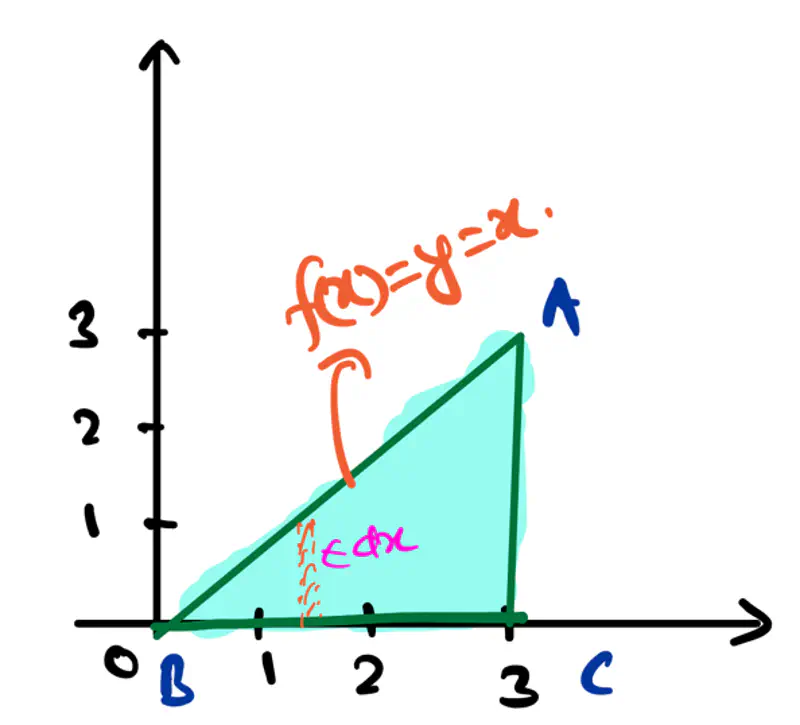
Integration is a mathematical tool that is used to find the area under a curve.

\[ \text{Area under the curve = } \int_{a}^{b} f(x) dx \\[10pt] and ~ \int x^n dx = \frac{x^{n+1}}{n+1} + C, \text{ where C is constant.} \\ \]

Let’s understand integration with the help of few simple examples for finding area under a curve:

Area of a triangle:
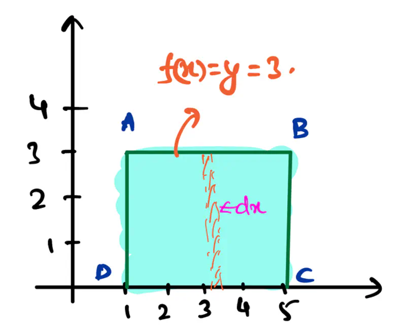
\[ \text{Area of } \triangle ~ABC = \frac{1}{2} \times base \times height = \frac{1}{2} \times 3 \times 3 = 9/2 = 4.5 \\[10pt] \text{Area of } \triangle ~ABC = \int_0^3 f(x) dx = \int_0^3 x dx = \frac{x^2}{2} \big|_0^3 = \frac{3^2 - 0^2}{2} = 9/2 = 4.5 \]
Area of a rectangle:
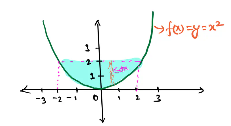
\[ \text{Area of rectangle ABCD} = length \times breadth = 4 \times 3 = 12 \\[10pt] \text{Area of rectangle ABCD} = \int_1^5 f(x) dx = \int_1^5 3 dx = 3x \big|_1^5 = 3(5-1) = 12 \]

Note: The above examples were standard straight forward, where we know a direct formula for finding area under a curve.
But, what if we have such a shape, for which, we do NOT know a ready-made formula, then how do we calculate the area under the curve.
Let’s see an example:

3. Area of a part of parabola:

\[ \text{Area under curve} = \int_{-2}^2 f(x) dx = \int_{-2}^2 x^2 dx = \frac{x^3}{3} \big|_{-2}^2 = \frac{(2)^3 - (-2)^3}{3} = \frac{8 - (-8)}{3} = \frac{16}{3} \]

Watch Video

Differentiation

Differentiation is a mathematical tool that is used to find the derivative or rate of change of a function at a specific point.

\(\frac{dy}{dx} = f\prime(x) = tan\theta\) = Derivative = Slope = Gradient
Derivative tells us how fast the function is changing at a specific point in relation to another variable.

Note: For a line, the slope is constant, but for a parabola, the slope is changing at every point.

How do we calculate the slope at a given point?

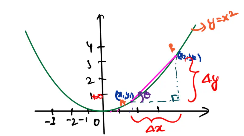
Let AB is a secant on the parabola, i.e, line connecting any 2 points on the curve.
Slope of secant = \(tan\theta = \frac{\Delta y}{\Delta x} = \frac{y_2-y_1}{x_2-x_1}\)
As \(\Delta x \rightarrow 0\), secant will become a tangent to the curve, i.e, the line will touch the curve only at 1 point.
\(dx = \Delta x \rightarrow 0\)
\(x_2 = x_1 + \Delta x \)
\(y_2 = f(x_2) = f(x_1 + \Delta x) \)
Slope at \(x_1\) =

\[ tan \theta = \frac{y_2-y_1}{x_2-x_1} = \frac{f(x_1 + \Delta x) - f(x_1)}{(x_1 + \Delta x)-x_1} \\[10pt] \therefore tan \theta = \lim_{\Delta x \rightarrow 0} \frac{f(x_1 + \Delta x) - f(x_1)}{\Delta x} \\[10pt] Generally, ~ slope = ~ tan \theta = \frac{dy}{dx} = \lim_{\Delta x \rightarrow 0} \frac{f(x + \Delta x) - f(x)}{\Delta x} \]

e.g.:
\( y = f(x) = x^2\), find the derivative of f(x) w.r.t x.

\[ \begin{aligned} \frac{dy}{dx} &= \lim_{\Delta x \rightarrow 0} \frac{f(x + \Delta x) - f(x)}{\Delta x} \\[10pt] &= \lim_{\Delta x \rightarrow 0} \frac{(x + \Delta x)^2 - x^2}{\Delta x} \\[10pt] &= \lim_{\Delta x \rightarrow 0} \frac{\cancel {x^2} + (\Delta x)^2 + 2x\Delta x - \cancel {x^2}}{\Delta x} \\[10pt] &= \lim_{\Delta x \rightarrow 0} \frac{\cancel {\Delta x}(\Delta x + 2x)}{\cancel {\Delta x}} \\[10pt] \text {applying limit: } \\ \therefore \frac{dy}{dx} &= 2x \\[10pt] \end{aligned} \]

Rules of Differentiation

We will understand few important rules of differentiation that are most frequently used in Machine Learning.

Sum Rule:
\[ \frac{d}{dx} (f(x) + g(x)) = \frac{d}{dx} f(x) + \frac{d}{dx} g(x) = f\prime(x) + g\prime(x) \]
Product Rule:
\[ \frac{d}{dx} (f(x).g(x)) = \frac{d}{dx} f(x).g(x) + f(x).\frac{d}{dx} g(x) = f\prime(x).g(x) + f(x).g\prime(x) \]
e.g.:
\( h(x) = x^2 sin(x) \), find the derivative of h(x) w.r.t x.
Let, \(f(x) = x^2 , g(x) = sin(x)\).
\[ h(x) = f(x).g(x) \\[10pt] => h\prime(x) = f\prime(x).g(x) + f(x).g\prime(x) \\[10pt] => h\prime(x) = 2x.sin(x) + x^2.cos(x) \\[10pt] \]
Quotient Rule:
\[ \frac{d}{dx} \frac{f(x)}{g(x)} = \frac{f\prime(x).g(x) - f(x).g\prime(x)}{(g(x))^2} \]
e.g.:
\( h(x) = sin(x)/x \), find the derivative of h(x) w.r.t x.
Let, \(f(x) = sin(x) , g(x) = x\).
\[ h(x) = \frac{f(x)}{g(x)} \\[10pt] => h\prime(x) = \frac{f\prime(x).g(x) - f(x).g\prime(x)}{(g(x))^2} \\[10pt] => h\prime(x) = \frac{cos(x).x - sin(x)}{x^2} \\[10pt] \]
Chain Rule:
\[ \frac{d}{dx} (f(g(x))) = f\prime(g(x)).g\prime(x) \]
e.g.:
\( h(x) = log(x^2) \), find the derivative of h(x) w.r.t x.
Let, \( u = x^2 \)
\[ h(x) = log(u) \\[10pt] => h\prime(x) = \frac{d h(x)}{du} \cdot \frac{du}{dx} \\[10pt] => h\prime(x) = \frac{1}{u} \cdot 2x = \frac{2x}{x^2} \\[10pt] => h\prime(x) = \frac{2}{x} \]

Now, let’s dive deeper and understand the concepts that required for differentiation, such as, limits, continuity, differentiability, etc.

Limits

Limit of a function f(x) at any point ‘c’ is the value that f(x) approaches, as x gets very close to ‘c’,
but NOT necessarily equal to ‘c’.

One-sided limit: value of the function, as it approaches a point ‘c’ from only one direction, either left or right.
Two-sided limit: value of the function, as it approaches a point ‘c’ from both directions, left and right, simultaneously.

e.g.:

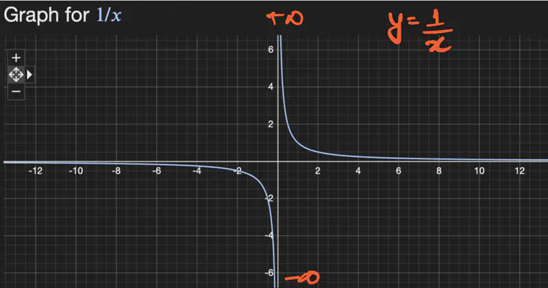
\(f(x) = \frac{1}{x}\), find the limit of f(x) at x = 0.
Let’s check for one-sided limit at x=0:
\[ \lim_{x \rightarrow 0^+} \frac{1}{x} = + \infty \\[10pt] \lim_{x \rightarrow 0^-} \frac{1}{x} = - \infty \\[10pt] so, \lim_{x \rightarrow 0^+} \frac{1}{x} ⍯ \lim_{x \rightarrow 0^-} \frac{1}{x} \\[10pt] => \text{ limit does NOT exist at } x = 0. \]
\(f(x) = x^2\), find the limit of f(x) at x = 0.
Let’s check for one-sided limit at x=0:
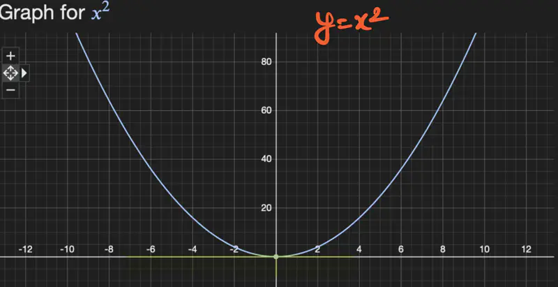
\[ \lim_{x \rightarrow 0^+} x^2 = 0 \\[10pt] \lim_{x \rightarrow 0^-} x^2 = 0 \\[10pt] so, \lim_{x \rightarrow 0^+} x^2 = \lim_{x \rightarrow 0^-} x^2 \\[10pt] => \text{ limit exists at } x = 0. \]

Note: Two-Sided Limit
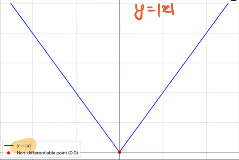
\[ \lim_{x \rightarrow a^+} f(x) = \lim_{x \rightarrow a^-} f(x) = \lim_{x \rightarrow a} f(x) \]
f(x) = |x|, find the limit of f(x) at x = 0.
Let’s check for one-sided limit at x=0:
\[ \lim_{x \rightarrow 0^+} |x| = x = 0 \\[10pt] \lim_{x \rightarrow 0^-} |x| = -x = 0 \\[10pt] so, \lim_{x \rightarrow 0^+} |x| = \lim_{x \rightarrow 0^-} |x| \\[10pt] => \text{ limit exists at } x = 0. \]

Continuity

A function f(x) is said to be continuous at a point ‘c’, if its graph can be drawn through that point, without lifting the pen.
Continuity bridges the gap between the function’s value at the given point and the limit.

Conditions for Continuity:
A function f(x) is continuous at a point ‘c’, if and only if, all the below 3 conditions are met:

f(x) must be defined at point ‘c’.
Limit of f(x) must exist at point ‘c’, i.e, left and right limits must be equal. \[ \lim_{x \rightarrow c^+} f(x) = \lim_{x \rightarrow c^-} f(x) \]
Value of f(x) at ‘c’ must be equal to its limit at ‘c’. \[ \lim_{x \rightarrow c} f(x) = f(c) \]

e.g.:

\(f(x) = \frac{1}{x}\) is NOT continuous at x = 0, since, f(x) is not defined at x = 0.
\(f(x) = |x|\) is continuous everywhere.
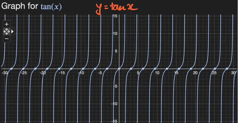
\(f(x) = tanx \) is discontinuous at infinite points.

Differentiability

A function is differentiable at a point ‘c’, if derivative of the function exists at that point.
A function must be continuous at the given point ‘c’ to be differentiable at that point.
Note: A function can be continuous at a given point, but NOT differentiable at that point.

\[ f\prime(x) = \lim_{\Delta x \rightarrow 0} \frac{f(x + \Delta x) - f(x)}{\Delta x} \]

e.g.:
We know that \( f(x) = |x| \) is continuous at x=0, but its NOT differentiable at x=0.

\[ f\prime(x) =\lim_{\Delta x \rightarrow 0} \frac{f(x + \Delta x) - f(x)}{\Delta x} = \lim_{\Delta x \rightarrow 0} \frac{|x + \Delta x| - |x|}{\Delta x} \\[10pt] \text{ let's calculate the one-sided limit from both left and right sides and check if they are equal: } \\[10pt] if ~ x>0, \lim_{\Delta x \rightarrow 0^+} \frac{|x + \Delta x| - |x|}{\Delta x} = \lim_{\Delta x \rightarrow 0+} \frac{\cancel x + \Delta x - \cancel x}{\Delta x} = 1 \\[10pt] if ~ x<0, \lim_{\Delta x \rightarrow 0^-} \frac{|x + \Delta x| - |x|}{\Delta x} = \lim_{\Delta x \rightarrow 0^-} \frac{-(x + \Delta x) - (-x)}{\Delta x} = \lim_{\Delta x \rightarrow 0-} \frac{\cancel {-x} - \Delta x + \cancel x}{\Delta x} = -1 \\[10pt] => \text{ left hand limit (-1) ⍯ right hand limit (1) } \\[10pt] => f\prime(0) \text{ does NOT exist.} \]

Maxima & Minima

Critical Point:
A point of the function where the derivative is either zero or undefined.

These critical points are candidates for local maxima or minima, which are the highest and lowest points in a function’s immediate neighborhood, respectively.

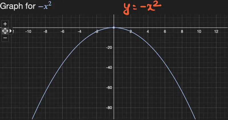
Maxima:
Highest point w.r.t immediate neighbourhood.
f’(x)/gradient/slope changes from +ve to 0 to -ve, therefore, change in f’(x) is -ve.
=> f’’(x) < 0

Let, \(f(x) = -x^2; \quad f'(x) = -2x; \quad f''(x) = -2 < 0 => maxima\)

x	f’(x)
-1	2
0	0
1	-2

Minima:
Lowest point w.r.t immediate neighbourhood.
f’(x)/gradient/slope changes from -ve to 0 to +ve, therefore, change in f’(x) is +ve.
=> f’’(x) > 0

Let, \(f(x) = x^2; \quad f'(x) = 2x; \quad f''(x) = 2 > 0 => minima\)

x	f’(x)
-1	-2
0	0
1	2

e.g.:

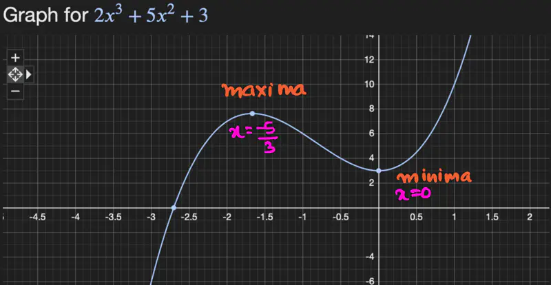
Let \(f(x) = 2x^3 + 5x^2 + 3 \), find the maxima and minima of f(x).
To find the maxima and minima, lets take the derivative of the function and equate it to zero.
\[ f'(x) = 6x^2 + 10x = 0\\[10pt] => x(6x+10) = 0 \\[10pt] => x = 0 \quad or \quad x = -10/6 = -5/3 \\[10pt] \text{ lets check the second order derivative to find which point is maxima and minima: } \\[10pt] f''(x) = 12x + 10 \\[10pt] => at ~ x = 0, \quad f''(x) = 12*0 + 10 = 10 >0 \quad => minima \\[10pt] => at ~ x = -5/3, \quad f''(x) = 12*(-5/3) + 10 = -20 + 10 = -10<0 \quad => maxima \\[10pt] \]
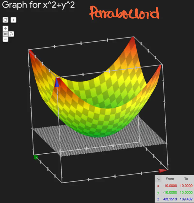
\(f(x,y) = z = x^2 + y^2\), find the minima of f(x,y).
Since, this is a multi-variable function, we will use vector and matrix for calculation.
\[ Gradient = \nabla f_z = \begin{bmatrix} \frac{\partial f_z}{\partial x} \\ \\ \frac{\partial f_z}{\partial y} \end{bmatrix} = \begin{bmatrix} 2x \\ \\ 2y \end{bmatrix} = \begin{bmatrix} 0 \\ \\ 0 \end{bmatrix} \\[10pt] => x=0, y=0 \text{ is a point of optima for } f(x,y) \]

Partial Derivative:
Partial derivative \( \frac{\partial f(x,y)}{\partial x} ~or~ \frac{\partial f(x,y)}{\partial y} \)is the rate of change or derivative of a multi-variable function w.r.t one of its variables, while all the other variables are held constant.

Let’s continue solving the above problem, and calculate the Hessian, i.e, 2nd order derivative of f(x,y):

\[ Hessian = H_z = \begin{bmatrix} \frac{\partial^2 f_z}{\partial x^2} & \frac{\partial^2 f_z}{\partial x \partial y} \\ \\ \frac{\partial^2 f_z}{\partial y \partial x} & \frac{\partial^2 f_z}{\partial y^2} \end{bmatrix} = \begin{bmatrix} 2 & 0 \\ \\ 0 & 2 \end{bmatrix} \]

Since, determinant of Hessian = 4 > 0 and \( \frac{\partial^2 f_z}{\partial x^2} > 0\) => (x=0, y=0) is a point of minima.

Hessian Interpretation:

Minima: If det(Hessian) > 0 and \( \frac{\partial^2 f(x,y)}{\partial x^2} > 0\)
Maxima: If det(Hessian) > 0 and \( \frac{\partial^2 f(x,y)}{\partial x^2} < 0\)
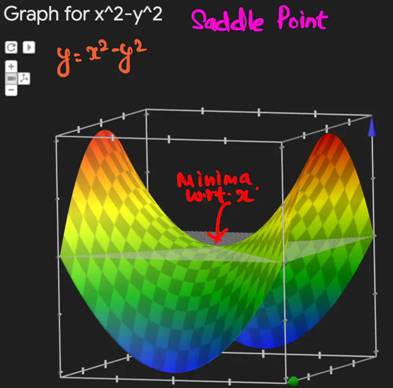
Saddle Point: If det(Hessian) < 0
Inconclusive: If det(Hessian) = 0, need to perform other tests.

Saddle Point

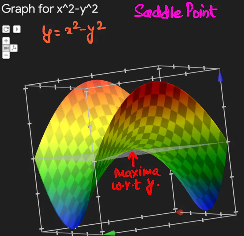
Saddle Point is a critical point where the function is maximum w.r.t one variable,
and minimum w.r.t to another.

e.g.:
Let, \(f(x,y) = z = x^2 - y^2\), find the point of optima for f(x,y).

\[ Gradient = \nabla f_z = \begin{bmatrix} \frac{\partial f_z}{\partial x} \\ \\ \frac{\partial f_z}{\partial y} \end{bmatrix} = \begin{bmatrix} 2x \\ \\ -2y \end{bmatrix} = \begin{bmatrix} 0 \\ \\ 0 \end{bmatrix} \\[10pt] => x=0, y=0 \text{ is a point of optima for } f(x,y) \]\[ Hessian = H_z = \begin{bmatrix} \frac{\partial^2 f_z}{\partial x^2} & \frac{\partial^2 f_z}{\partial x \partial y} \\ \\ \frac{\partial^2 f_z}{\partial y \partial x} & \frac{\partial^2 f_z}{\partial y^2} \end{bmatrix} = \begin{bmatrix} 2 & 0 \\ \\ 0 & -2 \end{bmatrix} \]

Since, determinant of Hessian = -4 < 0 => (x=0, y=0) is a saddle point.

Watch Video

End of Section