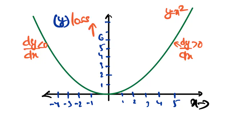
Gradient Descent

Gradient Descent for Optimization

3 minute read

In this section we will understand Gradient Descent for solving optimization problems in Machine Learning.

Calculus for AI & ML | Full Course Videos

Gradient Based Optimization

Till now, we have understood how to formulate a minimization problem as a mathematical optimization problem.
Now, lets take a step forward and understand how to solve these optimization problems.

We will focus on two important iterative gradient based methods:

Gradient Descent: First order method, uses only the gradient.
Newton’s Method: Second order method, used both the gradient and the Hessian.

📘

Gradient Descent:
It is a first order iterative optimization algorithm that is used to find the local minimum of a differentiable function.
It iteratively adjusts the parameters of the model in the direction opposite to the gradient of cost function, since moving opposite to the direction of gradient leads towards the minima.

Algorithm:

Initialize the weights/parameters with random values.
Calculate the gradient of the cost function at current parameter values.
Update the parameters using the gradient.
\[ w_{new} = w_{old} - \eta \cdot \frac{\partial f}{\partial w_{old}} \\[10pt] \eta: \text{ learning rate or step size to take for each parameter update} \]
Repeat steps 2 and 3 iteratively until convergence (to minima).

Types of Gradient Descent

There are 3 types of Gradient Descent:

Batch Gradient Descent
Stochastic Gradient Descent
Mini-Batch Gradient Descent

Batch Gradient Descent (BGD):
Computes the gradient using all the data points in the dataset for parameter update in each iteration.
Say, number of data points in the dataset is \(n\).
Let, the loss function for individual data point be \(l_i(w)\)

\[ l_i(w) = (y_i -\hat{y}_i)^2 \\[10pt] L(w) = \frac{1}{n} \sum_{i=1}^{n} l_i(w) \\[10pt] \frac{\partial L}{\partial w} = \frac{1}{n} \sum_{i=1}^{n} \frac{\partial l_i}{\partial w} \\[10pt] w_{new} = w_{old} - \eta \cdot \frac{\partial L}{\partial w_{old}} \\[10pt] w_{new} = w_{old} - \eta \cdot (\text{average of all 'n' gradients}) \]

Key Points:

Slow steps towards convergence, i.e, TC = O(n).
Smooth, direct path towards minima.
Number of steps/iterations is minimum.
Not suitable for large datasets; impractical for Deep Learning, as n = millions/billions.

Stochastic Gradient Descent (SGD):
It uses only 1 data point selected randomly from dataset to compute gradient for parameter update in each iteration.

\[ \frac{\partial L}{\partial w} \approx \frac{\partial l_i}{\partial w}, \text { say i = 5} \\[10pt] w_{new} = w_{old} - \eta \cdot (\text{gradient of i-th data point}) \]

Key Points:

Computationally fastest per step; TC = O(1).
Highly noisy, zig-zag path to minima.
High variance in gradient estimation makes path to minima volatile, requiring a careful decay of learning rate \(\eta\) to ensure convergence to minima.

Mini Batch Gradient Descent (MBGD):
It uses small randomly selected subsets of dataset, called mini-batch, (1<k<n) to compute gradient for parameter update in each iteration.

\[ \frac{\partial L}{\partial w} = \frac{1}{n} \sum_{i=1}^{k} \frac{\partial l_i}{\partial w} , \text { say k = 32} \\[10pt] w_{new} = w_{old} - \eta \cdot (\text{average gradient of k data points}) \]

Key Points:

Moderate time consumption per step; TC = O(k<n).
Less noisy, and more reliable convergence than stochastic gradient descent.
More efficient and faster than batch gradient descent.
Standard optimization algorithm for Deep Learning.
Note: Vectorization on GPUs allows for parallel processing of mini-batches; also GPUs are the reason for the mini-batch size to be a power of 2.

Watch Video

End of Section