Newton's Method
2 minute read
Newton’s Method:
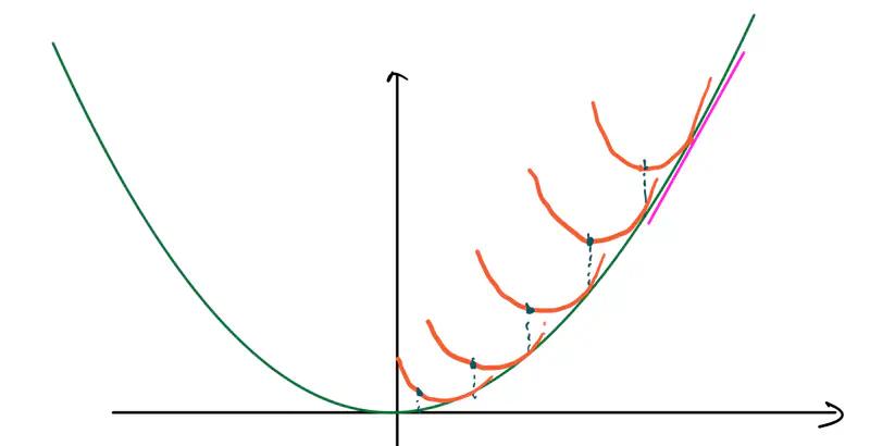
It is a second-order iterative gradient based optimization technique known for its extremely fast convergence.
When close to optimum, it achieves quadratic convergence, better than gradient descent’s linear convergence.
Algorithm:
- Start at a random point \(x_k\).
- Compute the slope at \(x_k, ~i.e,~ f'(x_k)\).
- Compute the curvature at \(x_k, ~i.e,~ f''(x_k)\).
- Draw a parabola at \(x_k\) that locally approximates the function.
- Jump directly to the minimum of that parabola; that’s the next step. Note: So, instead of walking down the slope step by step (gradient descent), we are jumping straight to the point where the curve bends downwards towards the bottom.

- Find the minima of \(f(x) = x^2 - 4x + 5\)
To find the minima, lets calulate the first derivative and equate to zero.
\(f'(x) = 2x - 4 = 0 \)
\( => x^* = 2 \)
\(f''(x) = 2 >0 \) => minima is at \(x^* = 2\)
Now, we will solve this using Newton’s Method.
Let’s start at x = 0.
Hence, we can see that using Newton’s Method we can get to the minima \(x^* = 2\) in just 1 step.
Full Newton’s Method is rarely used in Machine Learning/Deep Learning optimization,
because of the following limitations:
- \(TC = O(n^2\)) for Hessian calculation, since for a network with \(n\) parameters
requires \(n^2\) derivative calculations. - \(TC = O(n^3\)) for Hessian Inverse calculation.
- If it encounters a Saddle point, then it can go to a maxima rather than minima.
Because of the above limitations, we use Quasi-Newton methods like BFGS and L-BFGS.
The quasi-Newton methods make use of approximations for Hessian calculation, in order to gain the benefits
of curvature without incurring the cost of Hessian calculation.
BFGS: Broyden-Fletcher-Goldfarb-Shanno
L-BFGS: Limited-memory BFGS
End of Section