Optimization
8 minute read
How do we measure and minimize these mistakes in predictions made by the model?
minimizing a loss function.
Loss Function:
It quantifies error of a single data point in a dataset.
e.g.: Squared Loss, Hinge Loss, Absolute Loss, etc, for a single data point.
Cost Function:
It is the average of all losses over the entire dataset.
e.g.: Mean Squared Error(MSE), Mean Absolute Error(MAE), etc.
Objective Function:
It is the over-arching objective of an optimization problem, representing the function that is minimized or maximized.
e.g.: Minimize MSE.
Let’s understant this through an example:
Task:
Predict the price of a company’s stock based on its historical data.
Objective Function:
Minimize the difference between actual and predicted price.
Let, \(y\): original or actual price
\(\hat y\): predicted price
Say, the dataset has ’n’ such data points.
Loss Function:
loss = \( y - \hat y \) for a single data point.
We want to minimize the loss for all ’n’ data points.
Cost Function:
We want to minimize the average/total loss over all ’n’ data points.
So, what are the ways ?
- We take a simple sum of all the losses, but this can be misleading, as loss for a
single data point can be +ve or -ve, we can get a net-zero loss even for very large losses, when we sum them all. - We take the sum of absolute value of each loss, i.e, \( |y - \hat y| \), this way the losses will not cancel out each other.
But the absolute value function is NOT differentiable at y=0, and this can cause issues in optimisation algorithms, such as, gradient descent.
Read more about Differentiability - So, we choose squared loss, i.e, \( (y - \hat y)^2 \), this solves the above issues.
Note: In general, we refer to the cost function as the loss function also, the terms are used interchangeably.
Cost = Loss = Mean Squared Error(MSE) \[\frac{1}{n} \sum_{i=1}^{n} (y_i - \hat y_i)^2 \] The task is to minimize the above loss.
Key Points:
- Loss is the bridge between ‘data’ and ‘optimization’.
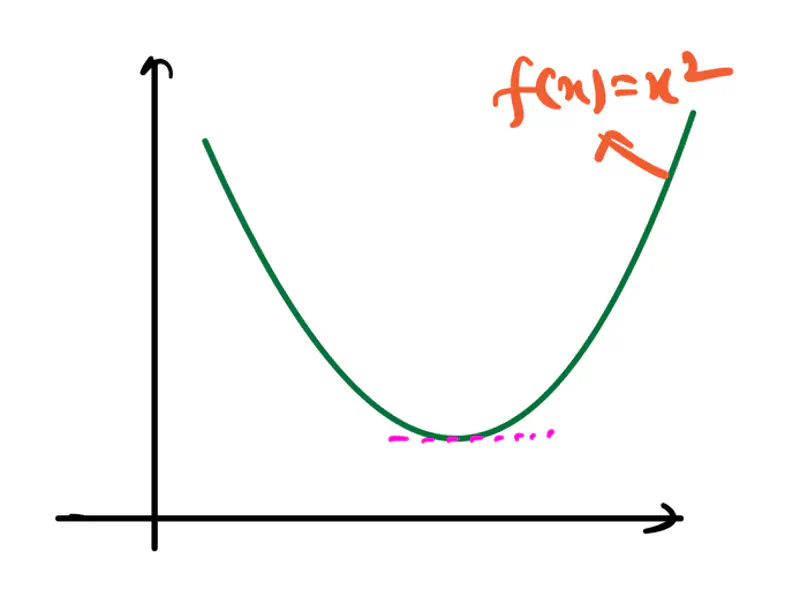
- Good loss functions are differentiable and convex.
Convexity:
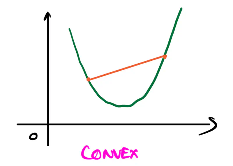
It refers to a property of a function where a line segment connecting any two points on its graph
lies above or on the graph itself.
A convex function is curved upwards.
It is always described by a convex set.


Convex Set:
A convex set is a set of points in which the straight line segment connecting any two points in the set lies
entirely within that set.
A set \(C\) is convex if for any two points \(x\) and \(y\) in \(C\), the convex combination
\(\theta x+(1-\theta )y\) is also in \(C\) for all values of \(\theta \) where \(0\le \theta \le 1\).
A function \(f: \mathbb{R}^n \rightarrow \mathbb{R}\) is convex if for all values of \(x,y\) and \(0\le \theta \le 1\),
\[ f(\theta x + (1-\theta )y) \le \theta f(x) + (1-\theta )f(y) \]Second-Order Test:
If a function is twice differentiable, i.e, 2nd derivative exists, then the function is convex,
if and only if, the Hessian is positive semi-definite for all points in its domain.
Positive Definite:
A symmetric matrix is positive definite if and only if:
- Eigenvalues are all strictly positive, or
- For any non-zero vector \(z\), the quadratic form \(z^THz > 0\)
Note: If the Hessian is positive definite, then the function is convex; has upward curvature in all directions.
Positive Semi-Definite:
A symmetric matrix is positive semi-definite if and only if:
- Eigenvalues are all non-negative (i.e, greater than or equal to zero), or
- For any non-zero vector \(z\), the quadratic form \(z^THz \ge 0\)
Note: If the Hessian is positive definite, then the function is not strictly convex, but flat in some directions.
All machine learning algorithms minimize loss (mostly), so we need to find the optimum parameters for the model that
minimizes the loss.
This is an optimization problem, i.e, find the best solution from a set of alternatives.
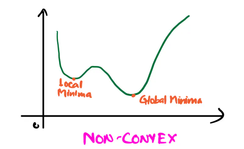
Note: Convexity ensures that there is only 1 minima for the loss function.
Optimization:
It is the iterative procedure of finding the optimum parameter \(x^*\) that minimizes the loss function f(x).
Let’s formulate an optimization problem for a model to minimize the MSE loss function discussed above:
Note: To minimize the loss, we want \(y_i, \hat y_i\) to be as close as possible, for that we want to find the optimum weights \(w, w_0\) of the model.

Important:
Deep Learning models have non-convex loss function, so it is challenging to reach the global minima,
so any local minima is also a good enough solution.
Read more about Maxima-Minima
Constrained Optimization:
It is an optimization process to find the best possible solution (min or max), but within a set of limitations or
restrictions called constraints.
Constraints limit the range of acceptable values; they can be equality constraints or inequality constraints.
e.g.:
Minimize f(x) subject to following constraints:
Equality Constraints: \( g_i(x) = c_i \forall ~i \in \{1,2,3, \ldots, n\} \)
Inequality Constraints: \( h_j(x) \le d_j \forall ~j \in \{1,2,3, \ldots, m\}\)
Lagrangian Method:
Lagrangian method converts a constrained optimization problem to an unconstrained optimization problem,
by introducing a new variable called Lagrange multiplier (\(\lambda\)).
Note: Addition of Lagrangian function that incorporates the constraints,
makes the problem solvable using standard calculus.
e.g.:
Let f(x) be the objective function with single equality constraint \(g(x) = c\),
then the Lagrangian function \( \mathcal{L}\) is defined as:
Now, the above constrained optimization problem becomes an unconstrained optimization problem:
By solving the above unconstrained optimization problem,
we get the optimum solution for the original constrained problem.
Objective: To minimize the distance between point (x,y) on the line 2x + 3y = 13 and the origin (0,0).
distance, d = \(\sqrt{(x-0)^2 + (y-0)^2}\)
=> Objective function = minimize distance = \( \underset{x^*, y^*}{\mathrm{argmin}}\ f(x,y) =
\underset{x^*, y^*}{\mathrm{argmin}}\ x^2+y^2\)
Constraint: Point (x,y) must be on the line 2x + 3y = 13.
=> Constraint (equality) function = \(g(x,y) = 2x + 3y - 13 = 0\)
Lagragian function =
To find the optimum solution, we solve the below unconstrained optimization problem.
Take the derivative and equate it to zero.
Since, it is multi-variable function, we take the partial derivatives, w.r.t, x, y and \(\lambda\).
Now, we have 3 variables and 3 equations (1), (2) and (3), lets solve them.
Hence, the point (x=2, y=3) on the line 2x + 3y = 13 that is closest to the origin.
To solve the optimization problem, there are many methods, such as, analytical method, which gives the normal equation for the linear regression,
but we will discuss that method later in detail, when we have understood what is linear regression?
Normal Equation for linear regression:
X: Feature variables
y: Vector of all observed target values
End of Section