Eigen Value Decomposition
11 minute read
It tells us about the characteristic properties of a matrix.
Multiplying a vector by a matrix can change the direction or magnitude or both of the vector.
\( \mathbf{A} = \begin{bmatrix}
2 & 1 \\
\\
1 & 2
\end{bmatrix}
\),
\(\mathbf{u} = \begin{bmatrix} 0 \\ \\ 1 \\ \end{bmatrix}\),
\(\mathbf{v} = \begin{bmatrix} 1 \\ \\ 1 \\ \end{bmatrix}\)
\(\mathbf{Au} = \begin{bmatrix} 1 \\ \\ 2 \\ \end{bmatrix}\) , \(\quad\)
\(\mathbf{Av} = \begin{bmatrix} 3 \\ \\ 3 \\ \end{bmatrix}\)
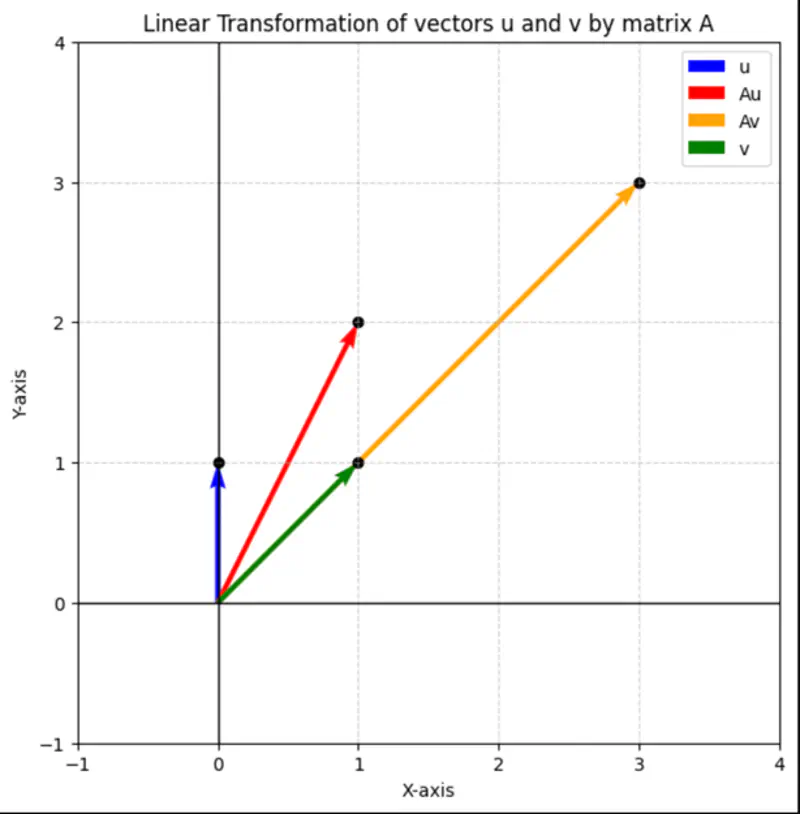
It might get scaled up or down but does not change its direction.
Result of linear transformation, i.e, multiplying the vector by a matrix, is just a scalar multiple of the original vector.
\(|\lambda| > 1 \): Vector stretched
\(0 < |\lambda| < 1 \): Vector shrunk
\(|\lambda| = 1 \): Same size
\(\lambda < 0 \): Vector’s direction is reversed
Since, for an eigen vector, result of linear transformation, i.e, multiplying the vector by a matrix, is just a scalar multiple of the original vector, =>
\[ \mathbf{A} \mathbf{v} = \lambda \mathbf{v} \\ \mathbf{A} \mathbf{v} - \lambda \mathbf{v} = 0 \\ \mathbf{v}(\mathbf{A} - \lambda \mathbf{I}) = 0 \\ \]For a non-zero eigen vector, \((\mathbf{A} - \lambda \mathbf{I})\) must be singular, i.e,
\(det(\mathbf{A} - \lambda \mathbf{I}) = 0 \)
If, \( \mathbf{A} =
\begin{bmatrix}
a_{11} & a_{12} & \cdots & a_{1n} \\
a_{21} & a_{22} & \cdots & a_{2n} \\
\vdots & \vdots & \ddots & \vdots \\
a_{n1} & a_{n2} & \cdots & a_{nn}
\end{bmatrix}
_{\text{n x n}}
\),
then, \((\mathbf{A} - \lambda \mathbf{I}) =
\begin{bmatrix}
a_{11}-\lambda & a_{12} & \cdots & a_{1n} \\
a_{21} & a_{22}-\lambda & \cdots & a_{2n} \\
\vdots & \vdots & \ddots & \vdots \\
a_{n1} & a_{n2} & \cdots & a_{nn}-\lambda
\end{bmatrix}
_{\text{n x n}}
\)
\(det(\mathbf{A} - \lambda \mathbf{I})) = 0 \), will give us a polynomial equation in \(\lambda\) of degree \(n\),
we need to solve this polynomial equation to get the \(n\) eigen values.
e.g.:
\( \mathbf{A} = \begin{bmatrix}
2 & 1 \\
\\
1 & 2
\end{bmatrix}
\),
\( \quad det(\mathbf{A} - \lambda \mathbf{I})) = 0 \quad \) =>
\( det \begin{bmatrix}
2-\lambda & 1 \\
\\
1 & 2-\lambda
\end{bmatrix} = 0
\)
\( (2-\lambda)^2 - 1 = 0\)
\( => |\lambda - 2| = \pm 1 \)
\( => \lambda_1 = 3\) and \( \lambda_2 = 1\)
Therefore, eigen vectors corresponding to eigen values \(\lambda_1 = 3\) and \( \lambda_2 = 1\) are:
\((\mathbf{A} - \lambda \mathbf{I}) \mathbf{v} = 0 \)
\(\lambda_1 = 3\)
=>
\(
\begin{bmatrix}
2-3 & 1 \\
\\
1 & 2-3
\end{bmatrix} \begin{bmatrix} v_1 \\ \\ v_2 \\ \end{bmatrix} =
\begin{bmatrix}
-1 & 1 \\
\\
1 & -1
\end{bmatrix} \begin{bmatrix} v_1 \\ \\ v_2 \\ \end{bmatrix} = 0
\)
=> Both the equations will be \(v_1 - v_2 = 0 \), i.e, \(v_1 = v_2\)
So, we can choose any vector, where x-axis and y-axis components are same, i.e, \(v_1 = v_2\)
=> Eigen vector: \(v_1 = \begin{bmatrix} 1 \\ \\ 1 \\ \end{bmatrix}\)
Similarly, for \(\lambda_2 = 1\)
we will get, eigen vector: \(v_2 = \begin{bmatrix} 1 \\ \\ -1 \\ \end{bmatrix}\)
\(\mathbf{Iv} = \lambda \mathbf{v}\)
Therefore, identity matrix has only one eigen value \(\lambda = 1\), and all non-zero vectors can be eigen vectors.
\(\mathbf{A} = \begin{bmatrix} 0 & 1 \\ \\ -1 & 0 \end{bmatrix} \), \( \quad det(\mathbf{A} - \lambda \mathbf{I}) = 0 \quad \) => det \(\begin{bmatrix} 0-\lambda & 1 \\ \\ -1 & 0-\lambda \end{bmatrix} = 0 \)
=> \(\lambda^2 + 1 = 0\) => \(\lambda = \pm i\)
So, eigen values are complex.
e.g.:
\( \mathbf{D} = \begin{bmatrix} d_{11} & 0 & \cdots & 0 \\ 0 & d_{22} & \cdots & 0 \\ \vdots & \vdots & \ddots & \vdots \\ 0 & 0 & \cdots & d_{nn} \end{bmatrix} _{\text{n x n}} \), \( \quad det(\mathbf{D} - \lambda \mathbf{I}) = 0 \quad \) => det \( \begin{bmatrix} d_{11}-\lambda & 0 & \cdots & 0 \\ 0 & d_{22}-\lambda & \cdots & 0 \\ \vdots & \vdots & \ddots & \vdots \\ 0 & 0 & \cdots & d_{nn}-\lambda \end{bmatrix} _{\text{n x n}} \)
=> \((d_{11}-\lambda)(d_{22}-\lambda) \cdots (d_{nn}-\lambda) = 0\)
=> \(\lambda = d_{11}, d_{22}, \cdots, d_{nn}\)
So, eigen values are the diagonal elements of the matrix.
- For a \(n \times n\) matrix, there are \(n\) eigen values.
- Eigen values need NOT be unique, e.g, identity matrix has only one eigen value \(\lambda = 1\).
- Sum of eigen values = trace of matrix = sum of diagonal elements, i.e,
\(tr(\mathbf{A}) = \lambda_1 + \lambda_2 + \cdots + \lambda_n\). - Product of eigen values = determinant of matrix, i.e,
\(det(\mathbf{A}) = |\mathbf{A}|= \lambda_1 \lambda_2 \cdots \lambda_n\). e.g: For the example matrix given above,
\( \mathbf{A} = \begin{bmatrix} 2 & 1 \\ \\ 1 & 2 \end{bmatrix} \), \(\quad \lambda_1 = 3\) and \( \lambda_2 = 1\)
\(tr(\mathbf{A}) = 2 + 2 = 3 + 1 = 4\)
\(det(\mathbf{A}) = 2 \times 2 - 1 \times 1 = 3 \times 1 = 3 \)
- Eigen vectors corresponding to distinct eigen values of a real symmetric matrix are orthogonal to each other.
Proof:
Let, \(\mathbf{v_1}, \mathbf{v_2}\) be eigen vectors corresponding to distinct eigen value \(\lambda_1,\lambda_2\) of a real symmetric matrix \(\mathbf{A} = \mathbf{A}^T\).
We know that for eigen vectors -
\[ \mathbf{Av_1} = \lambda_1 \mathbf{v_1} ~and~ \mathbf{Av_2} = \lambda_2 \mathbf{v_2} \\[10pt] \text{ let's calculate the dot product: } \\[10pt] \mathbf{Av_1} \cdot \mathbf{v_2} = (\mathbf{Av_1})^T\mathbf{v_2} = \mathbf{v_1^TA^Tv_2} = \mathbf{v_1^T} ~ \mathbf{Av_2}, \quad \text {since } \mathbf{A} = \mathbf{A}^T\\[10pt] => (\mathbf{Av_1}) \cdot \mathbf{v_2} = \mathbf{v_1} \cdot (\mathbf{Av_2}) \\[10pt] => (\lambda_1 \mathbf{v_1}) \cdot \mathbf{v_2} = \mathbf{v_1} \cdot (\lambda_2\mathbf{v_2}) \\[10pt] => \lambda_1 (\mathbf{v_1 \cdot v_2}) = \lambda_2 (\mathbf{v_1 \cdot v_2}) \\[10pt] => (\lambda_1 - \lambda_2) (\mathbf{v_1} \cdot \mathbf{v_2}) = 0 \\[10pt] \text{ since, eigen values are distinct,} => \lambda_1 ≠ \lambda_2 \\[10pt] \therefore \mathbf{v_1} \cdot \mathbf{v_2} = 0 \\[10pt] => \text{ eigen vectors are orthogonal to each other,} => \mathbf{v_1} \perp \mathbf{v_2} \\[10pt] \]
Let’ calculate the 2nd power of a square matrix.
e.g.:
\(\mathbf{A} = \begin{bmatrix}
2 & 1 \\
\\
1 & 2
\end{bmatrix}
\),
\(\quad \mathbf{A}^2 = \begin{bmatrix}
2 & 1 \\
\\
1 & 2
\end{bmatrix} \begin{bmatrix}
2 & 1 \\
\\
1 & 2
\end{bmatrix} = \begin{bmatrix}
5 & 4 \\
\\
4 & 5
\end{bmatrix}
\)
So, we need to find an easier way to calculate the power of a matrix.
Let’s calculate the 2nd power of a diagonal matrix.
e.g.:
\(\mathbf{A} = \begin{bmatrix}
3 & 0 \\
\\
0 & 2
\end{bmatrix}
\),
\(\quad \mathbf{A}^2 = \begin{bmatrix}
3 & 0 \\
\\
0 & 2
\end{bmatrix} \begin{bmatrix}
3 & 0 \\
\\
0 & 2
\end{bmatrix} = \begin{bmatrix}
9 & 0 \\
\\
0 & 4
\end{bmatrix}
\)
Note that when we square the diagonal matrix, then all the diagonal elements got squared.
Similarly, if we want to calculate the kth power of a diagonal matrix, then all we need to do is to just compute the kth
powers of all diagonal elements, instead of complex matrix multiplications.
\(\quad \mathbf{A}^k = \begin{bmatrix}
3^k & 0 \\
\\
0 & 2^k
\end{bmatrix}
\)
Therefore, if we diagonalize a square matrix then the computation of power of the matrix will become very easy.
Next, let’s see how to diagonalize a matrix.
\(\mathbf{V}\): Matrix of all eigen vectors(as columns) of matrix \(\mathbf{A}\)
\( \mathbf{V} = \begin{bmatrix}
\mathbf{v}_1 & \mathbf{v}_2 & \cdots & \mathbf{v}_n \\
\vdots & \vdots & \ddots & \vdots \\
\vdots & \vdots & \vdots & \vdots\\
\end{bmatrix}
\),
where, each column is an eigen vector corresponding to an eigen value \(\lambda_i\).
If \( \mathbf{v}_1 \mathbf{v}_2 \cdots \mathbf{v}_n \) are linearly independent, then,
\(det(\mathbf{V}) ~⍯ ~ 0\).
=> \(\mathbf{V}\) is NOT singular and \(\mathbf{V}^{-1}\) exists.
\(\Lambda\): Diagonal matrix of all eigen values of matrix \(\mathbf{A}\)
\( \Lambda = \begin{bmatrix}
\lambda_1 & 0 & \cdots & 0 \\
\\
0 & \lambda_2 & \cdots & 0 \\
\vdots & \vdots & \ddots & \vdots \\
0 & 0 & \cdots & \lambda_n
\end{bmatrix}
\),
where, each diagonal element is an eigen value corresponding to an eigen vector \(\mathbf{v}_i\).
Let’s recall the characteristic equation of a matrix for calculating eigen values:
\(\mathbf{A} \mathbf{v} = \lambda \mathbf{v}\)
Let’s use the consolidated matrix for eigen values and eigen vectors described above:
i.e, \(\mathbf{A} \mathbf{V} = \mathbf{\Lambda} \mathbf{V}\)
For diagonalisation:
=> \(\mathbf{\Lambda} = \mathbf{V}^{-1} \mathbf{A} \mathbf{V}\)
We can see that, using the above equation, we can represent the matrix \(\mathbf{A}\) as a
diagonal matrix \(\mathbf{\Lambda}\) using the matrix of eigen vectors \(\mathbf{V}\).
Just reshuffling the above equation will give us the Eigen Value Decomposition of the matrix \(\mathbf{A}\):
\(\mathbf{A} = \mathbf{V} \mathbf{\Lambda} \mathbf{V}^{-1}\)
Important: Given that \(\mathbf{V}^{-1}\) exists, i.e, all the eigen vectors are linearly independent.
Let’s revisit the example given above:
\(\mathbf{A} = \begin{bmatrix}
2 & 1 \\
\\
1 & 2
\end{bmatrix}
\),
\(\quad \lambda_1 = 3\) and \( \lambda_2 = 1\),
\(\mathbf{v_1} = \begin{bmatrix} 1 \\ \\ 1 \\ \end{bmatrix}\),
\(\mathbf{v_2} = \begin{bmatrix} 1 \\ \\ -1 \\ \end{bmatrix}\)
=> \( \mathbf{V} = \begin{bmatrix}
1 & 1 \\
\\
1 & -1 \\
\end{bmatrix}
\),
\(\quad \mathbf{\Lambda} = \begin{bmatrix}
3 & 0 \\
\\
0 & 1
\end{bmatrix}
\)
\( \because \mathbf{A} = \mathbf{V} \mathbf{\Lambda} \mathbf{V}^{-1}\)
We know, \( \mathbf{V} ~and~ \mathbf{\Lambda} \), we need to calculate \(\mathbf{V}^{-1}\).
\(\mathbf{V}^{-1} = \frac{1}{2}\begin{bmatrix} 1 & 1 \\ \\ 1 & -1 \\ \end{bmatrix} \)
\( \therefore \mathbf{V} \mathbf{\Lambda} \mathbf{V}^{-1} = \begin{bmatrix}
1 & 1 \\
\\
1 & -1 \\
\end{bmatrix} \begin{bmatrix}
3 & 0 \\
\\
0 & 1
\end{bmatrix} \frac{1}{2}\begin{bmatrix}
1 & 1 \\
\\
1 & -1 \\
\end{bmatrix}
\)
\( = \frac{1}{2}
\begin{bmatrix}
3 & 1 \\
\\
3 & -1 \\
\end{bmatrix} \begin{bmatrix}
1 & 1 \\
\\
1 & -1 \\
\end{bmatrix} = \frac{1}{2}\begin{bmatrix}
4 & 2 \\
\\
2 & 4 \\
\end{bmatrix}
\)
\( = \begin{bmatrix}
2 & 1 \\
\\
1 & 2
\end{bmatrix} = \mathbf{A}
\)
Spectral decomposition is a specific type of eigendecomposition that applies to a symmetric matrix,
requiring its eigenvectors to be orthogonal.
In contrast, a general eigendecomposition applies to any diagonalizable matrix and does not require the eigenvectors
to be orthogonal.
The eigen vectors corresponding to distinct eigen values are orthogonal.
However, the matrix \(\mathbf{V}\) formed by the eigen vectors as columns is NOT orthogonal,
because the rows/columns are NOT orthonormal i.e unit length.
So, in order to make the matrix \(\mathbf{V}\) orthogonal, we need to normalize the rows/columns of the matrix
\(\mathbf{V}\), i.e, make, each eigen vector(column) unit length, by dividing the vector by its magnitude.
After normalisation we get orthogonal matrix \(\mathbf{Q}\) that is composed of unit length and orthogonal eigen vectors
or orthonormal eigen vectors.
Since, matrix \(\mathbf{Q}\) is orthogonal, => \(\mathbf{Q}^T = \mathbf{Q}^{-1}\)
The eigen value decomposition of a square matrix is:
\(\mathbf{A} = \mathbf{V} \mathbf{\Lambda} \mathbf{V}^{-1}\)
And, the spectral decomposition of a real symmetric matrix is:
\(\mathbf{A} = \mathbf{Q} \mathbf{\Lambda} \mathbf{Q}^T\)
Important: Note that, we are discussing only the special case of real symmetric matrix here,
because a real symmetric matrix is guaranteed to have all real eigenvalues.
- Principal Component Analysis (PCA): For dimensionality reduction.
- Page Rank Algorithm: For finding the importance of a web page.
- Structural Engineering: By calculating the eigen values of a bridge’s structural model, we can identify its natural frequencies to ensure that the bridge won’t resonate and be damaged by external forces, such as wind, and seismic waves.
End of Section