Principal Component Analysis

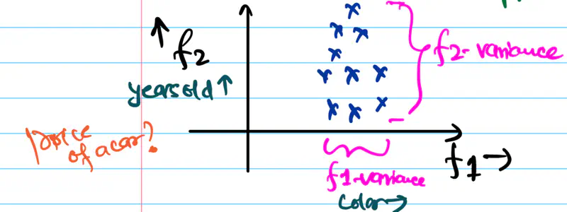
💡 In the diagram below, if we need to reduce the dimensionality of the data to 1, which feature should be dropped?

Whenever we want to reduce the dimensionality of the data, we should aim to minimize information loss.
Since, information = variance, we should drop the feature that brings least information, i.e, has least variance.
Therefore, drop the feature 1.

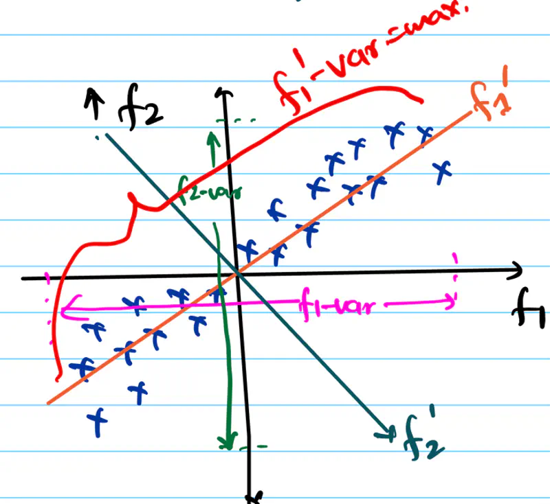
💡 What if the variance in both directions is same ?
What should be done in this case? Check the diagram below.

Here, since the variance in both directions is approximately same, in order to capture maximum variance in data,
we will rotate the f1-axis in the direction of maximum spread/variance of data, i.e, f1’-axis and then we can drop f2’-axis, which is perpendicular to f1’-axis.

📘

Principal Component Analysis (PCA)
It is a dimensionality reduction technique that finds the direction of maximum variance in the data.
Note: Some loss of information will always be there in dimensionality reduction, because there will be some variability in data along the direction that is dropped, and that will be lost.

Goal:
Fundamental goal of PCA is to find the new set of orthogonal axes, called the principal components, onto which the data can be projected, such that, the variance of the projected data is maximum.

Say, we have data, \(D:X \in \mathbb{R}^{n \times d}\),
n is the number of samples
d is the number of features or dimensions of each data point.
In order to find the directions of maximum variance in data, we will use the covariance matrix of data.
Covariance matrix (C) summarizes the spread and relationship of the data in the original d-dimensional space.
\(C_{d \times d} = \frac{1}{n-1}X^TX \), where \(X\) is the data matrix.
Note: (n-1) in the denominator is for unbiased estimation(Bessel’s correction) of covariance matrix.
\(C_{ii}\) is the variance of the \(i^{th}\) feature.
\(C_{ij}\) is the co-variance between feature \(i\) and feature \(j\).
Trace(C) = Sum of diagonal elements of C = Total variance of data.

Algorithm:

1. Data is first mean centered, i.e, make mean = 0, i.e, subtract mean from each data point.
   \(X = X - \mu\)
   

2. Compute the covariance matrix with mean centered data.
   \(C = \frac{1}{n-1}X^TX \), \( \quad \Sigma = \begin{bmatrix} var(f_1) & cov(f_1f_2) & \cdots & cov(f_1f_d) \\ cov(f_2f_1) & var(f_2) & \cdots & cov(f_2f_d) \\ \vdots & \vdots & \ddots & \vdots \\ cov(f_df_1) & cov(f_df_2) & \cdots & var(f_d) \end{bmatrix} _{\text{d x d}} \)

3. Perform the eigen value decomposition of covariance matrix.
   \( C = Q \Lambda Q^T \)
   \(C\): Orthogonal matrix of eigen vectors of covariance matrix.
   New rotated axes or prinicipal components of the data.
   \(\Lambda\): Diagonal matrix of eigen values of covariance matrix.
   Scaling of variance along new eigen basis.
   Note: Eigen values are sorted in descending order, i.e \( \lambda_1 \geq \lambda_2 \geq \cdots \geq \lambda_d \).
   

4. Project the data onto the new axes or principal components/directions.
   Note: k < d = reduced dimensionality.
   \(X_{new} = Z = XQ_k\)
   \(X_{new}\): Projected data or principal component score
   

💡 What is the variance of the projected data?

Variance of projected data is given by the eigen value of the co-variance matrix.
Covariance of projected data = \((XQ)^TXQ \)

\[ \begin{aligned} (XQ)^TXQ &= Q^TX^TXQ, \quad \text{ since, } (AB)^T = B^TA^T \\ &= Q^TQ \Lambda Q^TQ, \quad \text{ since, } C = X^TX = Q \Lambda Q^T \\ &= \Lambda, \quad \text{ since Q is orthogonal, } Q^TQ = I \\ \end{aligned} \]

Therefore, the diagonal matrix \( \Lambda \) captures the variance along every principal component direction.