Singular Value Decomposition

Singular Value Decomposition (SVD):
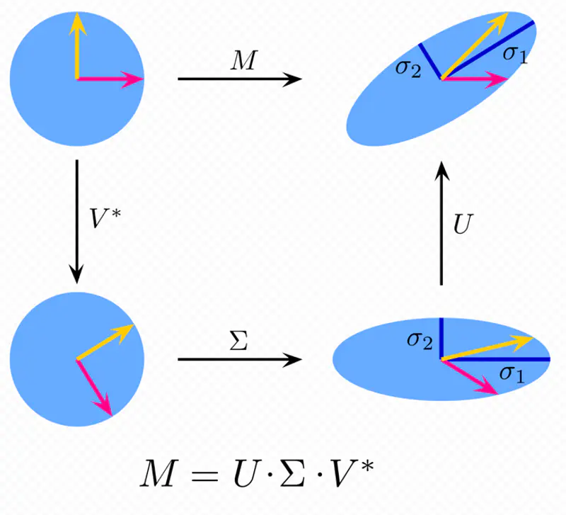
It decomposes any matrix into a rotation, a scaling (based on singular values), and another rotation.
It is a generalization of the eigen value decomposition(for square matrix) to rectangular matrices.
Any rectangular matrix can be decomposed into a product of three matrices using SVD, as follows:

\(\mathbf{U}\): Set of orthonormal eigen vectors of \(\mathbf{AA^T}_{m \times m} \)
\(\mathbf{V}\): Set of orthonormal eigen vectors of \(\mathbf{A^TA}_{n \times n} \)
\(\mathbf{\Sigma}\): Rectangular diagonal matrix, whose diagonal values are called singular values; square root of non-zero eigen values of \(\mathbf{AA^T}\).

Note: The number of non-zero diagonal entries in \(\mathbf{\Sigma}\) = rank of matrix \(\mathbf{A}\).
Rank (r): Number of linearly independent rows or columns of a matrix.

\( \Sigma = \begin{bmatrix} \sigma_{11} & 0 & \cdots & 0 \\ \\ 0 & \sigma_{22} & \cdots & 0 \\ \vdots & \vdots & \ddots & \vdots \\ \cdots & \cdots & \sigma_{rr} & \vdots \\ 0 & 0 & \cdots & 0 \end{bmatrix} \), such that, \(\sigma_{11} \geq \sigma_{22} \geq \cdots \geq \sigma_{rr}\), r = rank of \(\mathbf{A}\).

Singular value decomposition, thus refers to the set of scale factors \(\mathbf{\Sigma}\) that are fundamentally linked to the matrix’s singularity and rank.

We can perform singular value decomposition on the image matrix and find the minimum number of top ranks required to
to successfully reconstruct the original image back.
Say we performed the SVD on the image matrix and found that top 20 rank singular values, out of 1000, are sufficient to tell what the picture is about.

\(\mathbf{A} = \mathbf{U} \mathbf{\Sigma} \mathbf{V}^T \) \( = u_1 \sigma_1 v_1^T + u_2 \sigma_2 v_2^T + \cdots + u_r \sigma_r v_r^T \), where \(r = 20\)
A = sum of ‘r=20’ matrices of rank=1.
Now, we need to send only the \(u_i, \sigma_i , v_i\) values for i=20, i.e, top 20 ranks to earth
and then do the calculation to reconstruct the approximation of original image.
\(\mathbf{u} = \begin{bmatrix} u_1 \\ u_2 \\ \vdots \\ u_{1000} \end{bmatrix}\) \(\mathbf{v} = \begin{bmatrix} v_1 \\ v_2 \\ \vdots \\ v_{1000} \end{bmatrix}\)

So, we need to send data corresponding to 20 (rank=1) matrices, i.e, \(u_i, v_i ~and~ \sigma_i\) = (1000 + 1000 + 1)20 = 200020 pixels (approx)

Therefore, compression rate = (2000*20)/(10^6) = 1/25

Low Rank Approximation:
The process of approximating any matrix by a matrix of a lower rank, using singular value decomposition.
It is used for data compression.

Any matrix A of rank ‘r’ can be written as sum of rank=1 outer products:

\( \mathbf{u}_i : i^{th}\) column vector of \(\mathbf{U}\)
\( \mathbf{v}_i^T : i^{th}\) column vector of \(\mathbf{V}^T\)
\( \sigma_i : i^{th}\) singular value, i.e, diagonal entry of \(\mathbf{\Sigma}\)

Since, the singular values are arranged from largest to smallest, i.e, \(\sigma_1 \geq \sigma_2 \geq \cdots \geq \sigma_r\),
The top ranks capture the vast majority of the information or variance in the matrix.

So, in order to get the best rank-k approximation of the matrix, we simply truncate the summation after the k’th term.

The approximation \(\mathbf{A_k}\) is called the low rank approximation of \(\mathbf{A}\), which is achieved by keeping only the largest singular values and corresponding vectors.

Applications:

1. Image compression
2. Data compression, such as, LoRA (Low Rank Adaptation)