Cumulative Distribution Function
Cumulative Distribution Function of a Random Variable
5 minute read
In this section, we will understand Cumulative Distribution Function of a Random Variable.
📘 Random Variable(RV):
A random variable is a function that maps a the outcomes of a sample space to a real number.
Random Variable X represent as, \(X: \Omega \to \mathbb{R} \)
It maps abstract outcomes of a random experiment to concrete numerical values required for mathematical analysis.
A random variable is a function that maps a the outcomes of a sample space to a real number.
Random Variable X represent as, \(X: \Omega \to \mathbb{R} \)
It maps abstract outcomes of a random experiment to concrete numerical values required for mathematical analysis.
For example:
- Toss a coin 2 times, sample space: \(\Omega = \{HH,HT, TH, TT\}\)
The above random experiment of coin tosses can be mapped to a random variable \(X: \Omega \to \mathbb{R} \)
\(X: \Omega = \{HH,HT, TH, TT\} \to \mathbb{R}) \)
Say, if we count the number of heads, then
$$ \begin{aligned} X(0) = \{TT\} = 1 \\ X(1) = \{HT, TH\} = 2 \\ X(2) = \{HH\} = 1 \\ \end{aligned} $$ Similar, output will be observed for number of tails.
Depending upon the nature of output, random variables are of 2 types - Discrete and Continuous.
📘 Discrete Random Variable:
A random variable whose possible outcomes are finite or countably infinite.
Typically obtained by counting.
Discrete random variable cannot take any value between 2 consecutive values.
For example:A random variable whose possible outcomes are finite or countably infinite.
Typically obtained by counting.
Discrete random variable cannot take any value between 2 consecutive values.
- The number of heads in 2 coin tosses can be 0, 1 or 2 but NOT 1.5.
📘 Continuous Random Variable:
A random variable that can take any value between a given range/interval.
Possible outcomes are infinite.
For example:A random variable that can take any value between a given range/interval.
Possible outcomes are infinite.
- A person’s height in a given range of say 150cm-200cm.
Height can take any value, not just round values, e.g: 150.1cm, 167.95cm, 180.123cm etc.
Now, that we have understood that how random variable can be used to map outcomes of abstract random experiment to real
values for mathematical analysis, we will understand its applications.
💡 How to calculate the probability of a random variable?
Probability of a random variable is given by something called - Cumulative Distribution Function (CDF).
📘 Cumulative Distribution Function(CDF):
It gives the cumulative probability of a random variable \(X\).
CDF = \(F(X) = P(X \leq x)\) i.e Probability a random variable \(X\) will take for a value \(<=x\).
It gives the cumulative probability of a random variable \(X\).
CDF = \(F(X) = P(X \leq x)\) i.e Probability a random variable \(X\) will take for a value \(<=x\).
For example:
- Discrete random variable - Toss a coin 2 times, sample space: \(\Omega = \{HH,HT, TH, TT\}\)
Count the number of heads.
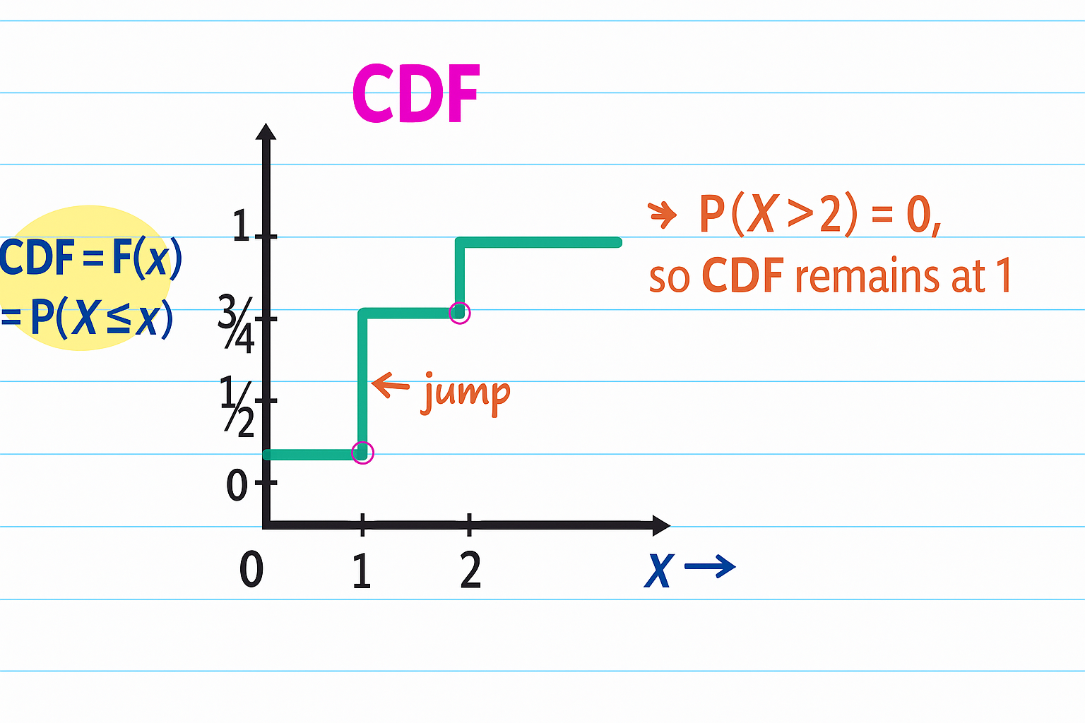
$$ \begin{aligned} X(0) = \{TT\} = 1 => P(X = 0) = 1/4 \\ X(1) = \{HT, TH\} = 2 => P(X = 1) = 1/2\\ X(2) = \{HH\} = 1 => P(X = 2) = 1/4 \\ \\ CDF = F(X) = P(X \leq x) \\ F(0) = P(X \leq 0) = P(X < 0) + P(X = 0) = 1/4 \\ F(1) = P(X \leq 1) = P(X < 1) + P(X = 1) = 1/4 + 1/2 = 3/4 \\ F(2) = P(X \leq 2) = P(X < 2) + P(X = 2) = 3/4 + 1/4 = 1 \\ \end{aligned} $$
2. Continuous random variable - Consider a line segment/interval from \(\Omega = [0,2] \)
Random variable \(X(\omega) = \omega\)
i.e \(X(1) = 1 ~and~ X(1.1) = 1.1 \)
Key properties of CDF
- Non-Decreasing:
For any 2 values \(x_1\) and \(x_2\) such that \(x_1 \leq x_2\), corresponding CDF must satisfy -
\(F(x_1) \leq F(x_2)\)
Note: Cumulative function can never decrease as x increases. - Bounded:
Range of CDF is always between 0 and 1, because CDF represents total probability, which cannot be negative or greater than 1.
\(\lim_{x \to -\infty} F(X) = 0\); as \(x \to -\infty\), event \((X \le x)\) becomes an impossible event
i.e \(P(X \le x) =0\)
\(\lim_{x \to \infty} F(X) = 1\); as \(x \to \infty\), event \((X \le x)\) includes all possible outcomes of the event, making sure that \(P(X \le x) =1\) - Right Continuous:
Function’s value at a point is same as the limit of the function, as we approach that point from right hand side (RHS).
Note: Reason for only right continuity is because how the cumulative distribution function is defined, as we may have a jump on the left side of the point.
\(\lim_{h \to o^+} F(X+h) = F(X)\)
For example:
In the above coin toss CDF example, if we approach X=1 from right, say 1.001, 1.01 etc, the value of \(F(X) = P(X \leq x) = F(1) = 3/4\).
But, if we approach \(X=1\) from left, say 0.99, 0.999 etc, the value of \(F(X) = 1/4\), as these values do NOT yet include the value of the probability at \(X=1\).
Discrete Case
For a discrete random variable, the CDF is a step function (i.e with jumps).Value of the probability of a random variable X, at any given value x, is calculated by summing up all the probabilities for values \(\le x\).
\( CDF = F_X(x) = \sum_{x_i \le x} P(X=x_i) \), where \(P(X=x_i)\) is the Probability Mass Function (PMF) at \(x_i\)
In the above coin toss example -
Height of the jump at ‘x’ = Probability at that value ‘x’.
e.g: Jump at (x=1) = 1/2 = Probability at (x=1).
Continuous Case
For a continuous random variable, the CDF is a continuous function.CDF for continuous random variable is calculated by integrating the probability density function (PDF) from \(-\infty\) to the given value \(x\).
\( CDF = F_X(x) = \int_{-\infty}^{x} f(x) \,dx \), where \(f(x)\) is the Probability Density Function (PDF) of random variable.
Note: We can also say that PDF is the derivative of CDF for continuous random variable.
\(PDF = f(x) = F'(X) = \frac{dF_X(x)}{dx} \)
End of Section